Gengo Girls #2: Hiragana Hijinks

Genki Gengo Girls #2: Hiragana Hijinks

<< Previous Comic

Next Comic >>

Other special rules you should know:

  • Adding a small circle to an “H” symbol turns it into a “P” symbol. Ex: は= ha, but ぱ= pa
  • If you follow a symbol up with a vowel that has the same sound, you double the length of the the first symbol and ignore the vowel. Ex: かあ is “kaa” not “ka (pause) a”
  • You can also double “O” sounds by using the う symbol instead of the お symbol. Ex: おう is pronounced as a long “oh” sound, not “oh-ew”

Transcript

Yellow: They say the Japanese alphabet only has forty six letters, but when you count the special rules isn’t it more like a hundred?

Blue: What do you mean?

Yellow: Well, there’s the way you can add the ” symbol to a letter to change K sounds into G sounds or H into B or S into Z or T into D. That’s like adding twenty more letters!

Blue: I guess that’s true. がんばる is “ganbaru” not “kanharu”

Yellow: And don’t forget that you can throw in a tiny や, よ, or ゆ after another symbol to mix the sounds together. That has to be worth another dozen letters!

Blue: That’s true too. りゅう is “ryuu” instead of “riyuu”.

Yellow: Woah! You can actually pronounce りゅう?!

Yellow: It always comes out “ruu” or “riyuu” when I try…

Blue: My brother took me to the arcade a lot as a kid…

Gengo Girls #1: Minimum System Requirements

Genki Gengo Girls 1: Minimum System Requirements

<< Previous Comic

Next Comic >>

Here is a link to the Wikipedia article on hiragana. I just saved you something like twenty three key strokes. You’re welcome.

I personally found that the easiest way to memorize hiragana, and later katakana, was to split them up into groups of five based on what kind of sound they made. First I learned all the “vowel” sounds (あ い う え お) and then all the “K” sounds (か き く け こ) and so on.

Transcript

Blue: Today I’m going to be talking about the things you need to know to fully enjoy this comic.

Yellow: Another “talking through the fourth wall gag? We did that last time.

Blue: It’s not a gag. The audience needs to hear this.

Blue: First off, you’re going to need to know how to read hiragana. It’s a 46 letter Japanese alphabet where each symbol represents a one-syllable sound.

Blue: We’ll use hiragana to teach you how to pronounce new words.

Yellow: It might also be useful to learn katakana. It’s an alternate alphabet used mostly for foreign words.

Yellow: Shows up in manga sound effects a lot too!

Blue: Memorizing 46 symbols isn’t all that hard. Just make some flash cards or look for an online tutorial!

Blue: You can do this!

Yellow: There are even phone apps for learning hiragana!? Wish I had known that BEFORE making all those flash cards…

Introducing Gengo Girls

Introducing Genki Gengo Girls

Next Comic >>

Obviously you can’t learn an entire language just from reading a four panel comic strip, but “Gengo Girls” will do its best to cover the basics and provide a fun way for more advanced students to review what they already know.


Transcript

Blue: What did you think of yesterday’s Japanese assignment?

Yellow: I kind of… didn’t do it.

Blue: Oh my. Was it too hard?

Yellow: More like too boring! I just can’t get interested in reading our textbook.

Blue: But how are you going to learn Japanese if you don’t read the textbook?

Yellow: Easy! I’ll just find a web comic about two cute girls explaining Japanese to each other.

Yellow: Now strike a pose for the fourth wall!

Blue: We’ll do our best to help you learn Japanese, but you really should read a textbook too.

Let’s Program A Swarm Intelligence: Index And Code

Introduction


Welcome fellow AI enthusiasts. Have you ever heard the phrase “Swarm Intelligence” and wondered just exactly what that means? Then wonder no more because I have here for you a whole set of articles about how to use swarm intelligence techniques to build a flexible AI capable of optimizing a wide variety of mathematical problems and real world equations.


Basically it all boils down to something like this:

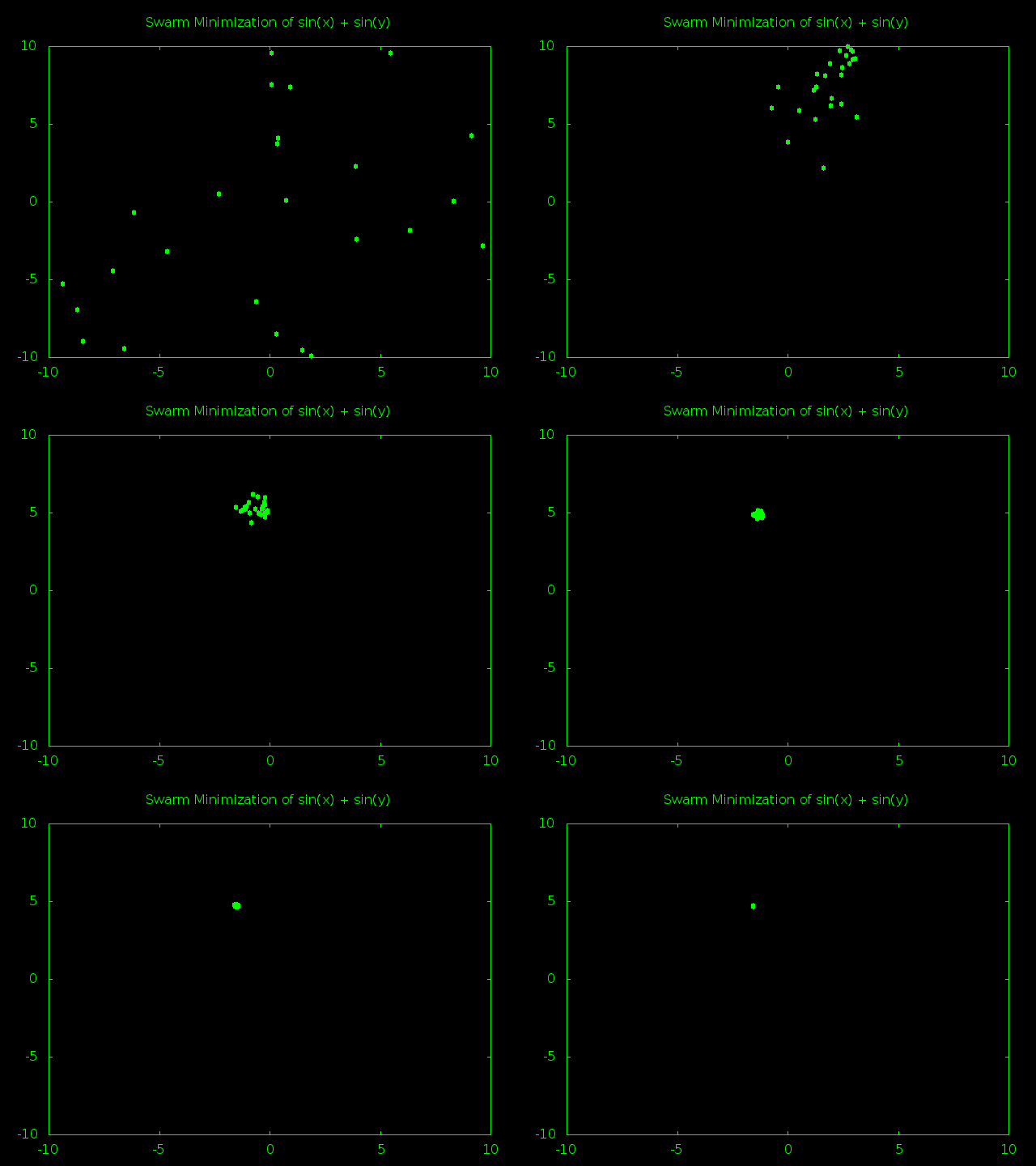
An animation of a swarm optimizing a sine wave based function

A really cool looking swarm intelligence


Index

Let’s Program A Swarm Intelligence 1: Introducing Particle Swarm Optimization

Let’s Program A Swarm Intelligence 2: Learning To Love Lisp

Let’s Program A Swarm Intelligence 3: All Your Max Are Min

Let’s Program A Swarm Intelligence 4: Specifying A Use Case

Let’s Program A Swarm Intelligence 5: Defining The Swarm

Let’s Program A Swarm Intelligence 6: Assembling The Swarm

Let’s Program A Swarm Intelligence 7: Satisfying My OCD

Let’s Program A Swarm Intelligence 8: It Lives!

Let’s Program A Swarm Intelligence 9: All Together Now

Let’s Program A Swarm Intelligence 10: Let Me See…

Let’s Program A Swarm Intelligence 11: Turning Your World Upside Down

Let’s Program A Swarm Intelligence 12: Is That A Trick Question?

Let’s Program A Swarm Intelligence 13: Welcome To The Nth Dimension

Let’s Program A Swarm Intelligence 14: Better Particles, Better Swarm

Let’s Program A Swarm Intelligence 15: The Return Of Maximize And Target

Let’s Program A Swarm Intelligence 16: The Swarm Ate My Homework


Complete Code

If you follow along with the posts you should be able to write your own swarm intelligence from scratch in whatever programming language you want. But if you don’t have the time for that or just want some reference code I have also provided my completed code: Lisp Swarm Intelligence

Let’s Program A Swarm Intelligence 16: The Swarm Ate My Homework

The Freshman Math Challenge


After roaming around on the Internet for a while I found a website offering open source college material including a rather decent worksheet on multi-variable optimization, which you can find here http://ocw.capilanou.ca/mathematics-statistics/math-109-calculus-ii/optimization-problems.pdf/view?searchterm=optimization.


I’ll be using problems from this worksheet to test out the swarm. Let’s see if we’ve built a machine smart enough to pass an entry level calculus class.


Profit Optimization


First problem from the worksheet is pretty straightforward. There is a random desk company that sells both finished and unfinished desks, although I’m not actually sure what they mean by this. Are they talking about whether or not the wood on the desk is properly stained, or by unfinished do they mean that they literally sell desks that are still missing pieces? Is there a big market for three legged desks?


Anyways, whatever an “unfinished” desk is the company’s revenue looks like this:


revenue = 200*finished + 160*unfinished – 0.2*finished*unfinished – 0.2*finished^2 – 0.25*unfinished^2.


The company’s expenses look like this


expense = 100*finished + 70*unfinished + 4000


The company’s profit is equal to its revenue minus its expenses, which we can represent as this Lisp function:


;Revenue for a company which sells both finished and unfinished furniture
(defun company-profit (fin unfin)
   (let ((revenue (+ (* 200 fin) 
                     (* 160 unfin) 
                     (* -0.2 fin unfin) 
                     (* -0.2 fin fin) 
                     (* -0.25 unfin unfin)))
         (expense (+ (* 100 fin) (* 70 unfin) 4000)))
      (- revenue expense)))


Now we just have to decide on some boundaries for our swarm guesses. Since you can’t produce less than 0 units of furniture our minimum bound for both types of desks will be 0. When it comes to the upper bounds we’ll have to take a bit of a guess. The bigger the boundary the larger our swarm will need to be to explore it and the longer the search will take, so we want to aim for an upper boundary that is small enough to be efficient while still being large enough to capture the maximum number of desks a company can reasonably build in one week.


Let’s start out with an upper bound of 10,000. That’s a pretty large number of desks for a small company to produce in a single week, so we should be safe. On the other hand, if that number is too small we’ll probably get an optimal solution right on the edge of our boundaries. If that happens we’ll just increase the boundaries and try again.


Now it’s time to put that all into action:


[5]> (defparameter *swarm-iterations* 200)

*SWARM-ITERATIONS*

[6]> (defparameter *swarm-size* 1000)

*SWARM-SIZE*

[7]> (defparameter *swarm-output* (swarm-maximize #’company-profit ‘((0 10000) (0 10000))))

*SWARM-OUTPUT*

[8]> (first *swarm-output*)

(200.04425 100.01073)


So it looks like the swarm thinks we should build 200 finished desks and 100 unfinished desks. And if we scroll down to the answer key portion of the worksheet that turns out to the right answer. Good job swarm!


Minimize Distances


Now let’s jump down to problem 3. A power station is being planned and they want to figure out the best place to put it so it can efficiently serve three different communities. Apparently this means they want to minimize the sum of the squares of the distances to each of the three communities which are positioned at (-4, 4) (5, 2) and (-1, -3).


Writing a function to calculate the sum of squares isn’t too hard, especially if we use the expt function to square things and the sqrt function to take square roots. Just remember that distance can be calculated by taking the square root of the square of the X and Y distances between two points and the following function should make perfect sense.


;Calculate the sum of squares of distances between a given point and the three points (-4, 4) (5, 2) and (-1, -3)
(defun sum-of-squared-distances (x y)
   (let ( (distance1 (sqrt (+ (expt (- x -4) 2) (expt (- y 4) 2))))
          (distance2 (sqrt (+ (expt (- x 5) 2) (expt (- y 2) 2))))
          (distance3 (sqrt (+ (expt (- x -1) 2) (expt (- y -3) 2)))))
      (+ (expt distance1 2) (expt distance2 2) (expt distance3 2))))


Time to choose our boundaries. Since we want to minimize the distance between the plant and the communities the power plant should logically be somewhere in the middle of the three points. So by looking at our points this means our x boundary needs to be between -4 and 5 and our y boundary needs to be between -3 and 4.


Time to let the swarm loose.


[29]> (defparameter *swarm-size* 25)

*SWARM-SIZE*

[30]> (defparameter *swarm-iterations* 100)

*SWARM-ITERATIONS*

[31]> (defparameter *swarm-output* (swarm-minimize #’sum-of-squared-distances ‘((-4 5) (-3 4))))

*SWARM-OUTPUT*

[32]> (first *swarm-output*)

(-7.074524E-4 1.0000945)


According to the swarm the best place for the power plant is around (0, 1), which matches up with the answer key. Another victory for the swarm!


A Problem With Extra Requirements


Now let’s go back to problem 2. This one turned out to be rather tricky.


At first it looks like a pretty simple. We have a package with length, width and depth (like all 3D objects). We want to maximize the volume. Just a simple 3 variable maximization, right?


Except that postal regulations require that the length and girth of the box have to add up to less than 108 inches. Or as the worksheet is happy to summarize: 2x + 2y + z <= 108.


This is a problem because our swarm is designed to make completely random guesses for x, y and z. We can give it some general guidelines like “x has to be between 0 and 10” but we can’t give it a complex constraint like “x plus y plus z needs to be less than 100”.


So at first it seems like our swarm just isn’t smart enough for this problem. But maybe there is a clever way around this issue. Take a look a this function:


;Calculates the volume of a package that has to have a combined length and girth of less than 108
(defun postal-package-volume (x y z)
   (if (> (+ (* 2 x) (* 2 y) z) 108)
       -1
       (* x y z)))


If the user tries to calculate the volume of a package that’s too big to mail we return -1 instead of the volume. Not only is this a good way to let a human know that there is a problem with their input, it also works great with our swarm. Since we want to maximize volume an “error” value of -1 will always be considered less optimal than even the worst of “acceptable” answers, all of which are positive.


In other words, instead of trying to prevent the swarm from making unacceptable guesses we just make sure that unacceptable guesses are always less optimal than acceptable guesses.


Time to see if it works. Our boundaries are based off the fact that a box can’t have negative length and that the definition of girth means that 54 is the biggest x and y values possible and that 108 is the biggest possible z.


[44]> (defparameter *swarm-size* 25)

*SWARM-SIZE*

[45]> (defparameter *swarm-iterations* 100)

*SWARM-ITERATIONS*

[46]> (defparameter *swarm-output* (swarm-maximize #’postal-package-volume ‘((0 54) (0 54) (0 108))))

*SWARM-OUTPUT*

[47]> (first *swarm-output*)

(17.743437 18.024296 36.464497)


If we look at the answer key the true maximum is (18, 18, 36), which is pretty close to the swarm’s guess. Looks like our workaround for the input constraints worked!


Conclusion And Extra Challenges


That’s it. We wrote a general swarm optimizer smart enough to ace a freshman calculus assignment. So while our swarm isn’t anywhere near being a professional quality artificial intelligence I think it’s more than good enough to be considered a successful “Let’s Program”.


Of course, I’m sure there are plenty of you out in the audience who don’t want to stop here. If you want to forge on ahead on your own here are a few sample projects you might want to consider tackling next:


  • Find more complicated optimization problems that require more than 3 variables. Does the swarm find the right answer? If not, fix it until it does.
  • Improve particle behavior by giving them memory of their personal best answer and having them adjust their velocity based on a combination of current velocity, swarm best and personal best.
  • Create multiple types of particles, such as scout particles that don’t care so much about the swarm best and random particles that bounce around problem space even when the rest of the swarm has settled on a possible best answer. This would be a great place to practice object oriented programming.


And with these final suggestions I bid you adieu. All that’s left is the index page. Thanks for following along!

Let’s Program A Swarm Intelligence 15: The Return of Maximize and Target

Solving A Problem We Already Solved


Last post we upgraded our swarm so that it could successfully minimize problems with any number of variables. All that’s left now is to teach it how to maximize and how to aim for specific results.


By now you should understand that maximization is just minimization turned upside down and hitting a target is the same as minimizing the difference between the results you are getting and the results you want.


Thanks to this insight we were able to easily write a 2D maximizer and target seeker by just using our already written minimizer. Now it’s time to do the same thing for the general swarm.


The tricky part here has to do with arguments.


In the 2D swarm we knew that everything would have two variables, so we were able to use lambda to build new two variable functions on demand. Then we passed that new two variable function to swarm-minimize-2d, which gave it the two arguments it expected.


But this time things are different. The general swarm-minimize uses apply to pass an unpredictable number of variables to our function. Which means that the new lambda function we build has to be able to accept a flexible number of variables and then pass them all on the the original function.


Fortunately for us Lisp is all ready to handle this problem thanks to the keyword &rest. Put inside of a function declaration this basically means “A list of every extra variable in the function call”.


A quick demo:


(defun rest-test (first second &rest extra)
   (format t “This is the first argument: ~a~%” first)
   (format t “This is the second argument: ~a~%” second)
   (format t “There were ~a extra arguments:~%” (length extra))
   (loop for argument in extra do (format t “~a~%” argument)))


[9]> (rest-test “one” “two” “three”)

This is the first argument: one

This is the second argument: two

There were 1 extra arguments:

three

NIL

[10]> (rest-test “one” “two” “three” “four” “five”)

This is the first argument: one

This is the second argument: two

There were 3 extra arguments:

three

four

five

NIL


This is exactly what we need in order to create a lambda function that can take a flexible number of variables and pass them all along to an inner function. Upgrading the 2D maximize and target functions is now simple:


(defun swarm-maximize (fn boundaries)
   (swarm-minimize (lambda (&rest arguments) (* -1 (apply fn arguments) boundaries))))

(defun swarm-target (fn target boundaries)
   (swarm-minimize-2d (lambda (&rest arguments) (abs (- target (apply fn arguments)))) boundaries))


Let’s take these new functions for a spin:


[16]> (defparameter *swarm-iterations* 100)

*SWARM-ITERATIONS*

[17]> (defparameter *swarm-output* (swarm-maximize #’inverse-double-parabola ‘((-10 10)(-10 10))))

*SWARM-OUTPUT*

[18]> (first *swarm-output*)

(5.114901E-5 4.665053E-7)

[19]> (defparameter *swarm-output* (swarm-target #’triple-parabola 7 ‘((-10 10)(-10 10)(-10 10))))

*SWARM-OUTPUT*

[20]> (first *swarm-output*)

(-1.5512012 0.78995675 -1.9924128)

[21]> (triple-parabola -1.5512012 0.78995675 -1.9924128)

6.9999657


Success on both counts!


Coincidentally, this also shows off that our general swarm optimizer can handle 2D problems just as well as the specific 2D swarm optimizer. This is nice because it let me test maximization on a function we already had and saved me the trouble of writing an inverse triple parabola.


Time To Give The Swarm A Real Run For It’s Money


Ok, so we were able to maximize and target a couple of parabolas using the general swarm. But that’s not really very impressive. Parabolas are easy to solve and these weren’t even high dimensional problems.


So for my next and final “Let’s Program A Swarm Intelligence” I’m going to pull out all the stops and try to find some real world multi-variable problems to test this thing on. I’m sure I have a few engineering and calculus textbooks laying around with interesting problems just waiting to be solved.


Let’s Program A Swarm Intelligence 14: Better Particles, Better Swarm

The End Is Near


Last time we successfully upgraded our particle objects to be flexible enough to work in any number of dimensions so they can help us optimize problems with any number of variables. Now all we need to do is upgrade our old 2D swarm algorithms to use these new super-particles and we’ll have a complete, generalized particle swarm optimizer.


Fair warning: A lot of the code in this post looks really complicated. And I guess it kind of is. But remember that everything we are doing in this post is something we’ve already done successfully in two dimensions and that the basic logic is the same. Just remember the basics of swarm logic (make a lot of guesses, update your guesses, repeat) and you should be fine.


Also, we can’t really develop a general swarm optimizer without a few multi-variable problems to test it on. So behold, Multi-dimensional parabolas!


(defun triple-parabola (x y z)
   (+ (* x x) (* y y) (* z z)))

(defun quadruple-parabola (x y z w)
   (+ (* x x) (* y y) (* z z) (* w w))


Once again the obvious minimum for both these problems is when all the inputs are set to 0. That’s (0, 0, 0) for the triple parabola and (0, 0, 0, 0) for the quadruple parabola. Hopefully the swarm will be able to figure that out too.


A More General Swarm Definition


The first step in upgrading our particles was to remove specific references to 2D ideas like X and Y and then replace them with flexible lists that can grow to whatever size the problem demands. Similarly the first step in upgrading the swarm itself is to remove specific 2D references and replace them with more flexible structures.


The big change here is that our 2D swarm used to keep track of the best X and Y coordinates any particle had found so far. We will now replace those with one “best-coordinates” variable that we will use to store a copy of the entire coordinates list of any particle that manages to find a good possible answer. This way we can have one variable that works no matter how long the coordinate list gets.


(defclass swarm ()
   ((best-coordinates
       :accessor best-coordinates
       :initform nil)
    (best-answer
       :initarg :best-answer
       :accessor best-answer
       :initform most-positive-long-float)
    (particle-list
       :accessor particle-list)))


Next up is creating a handy swarm generating function. Just like with the particle generator function the main focus of this upgrade will be to remove specific references to X and Y limits and replace them with a flexible “boundaries” list that will include a min and max pair for every variable in the problem we are minimizing.


(defun generate-swarm (particle-count boundaries)
   (let ((new-swarm (make-instance 'swarm)))
      (setf (particle-list new-swarm)
            (loop for i from 1 to particle-count
             collect (generate-particle boundaries)))
      new-swarm))


Most of the hard “boundaries” work was already done inside of generate-particle so this upgrade was as easy as swapping out a few old variables for a new one and making sure that “new-swarm” is created as a swarm object instead of a swarm-2d object.


Same Logic, More Numbers


Upgrading the swam logic is pretty easy. We just replace the idea of x-limit and y-limits with a single boundary variable and then switch to the non-2D version of every function call.


(defun swarm-minimize (fn boundaries)
   "A general particle swarm optimizer"
   (let ((swarm (generate-swarm *swarm-size* boundaries)))
      (loop for i from 1 to *swarm-iterations* do
         (loop for particle in (particle-list swarm)
           do (update-swarm-particle particle swarm fn boundaries)))
      (list (best-coordinates swarm) (get-swarm-history swarm))))


Only problem is… not all of these functions exist yet. So before swarm-minimize can actually be used for anything we’re going to have to write our new generic update-swarm-particle. Watch out because this one is a doozy!


(defun update-swarm-particle (particle swarm fn boundaries)
   (update-particle-history particle)
   (let ((particle-answer (apply fn (coordinates particle))))
      (when (< particle-answer (best-answer swarm))
         (setf (best-answer swarm) particle-answer)
         (setf (best-coordinates swarm) (coordinates particle))))
   (update-particle-velocity particle (best-coordinates swarm))
   (setf
      (coordinates particle)
      (loop
         for position in (coordinates particle)
         for velocity in (velocity particle)
         for bounds in boundaries
         collect (max (first bounds) (min (second bounds) (+ position velocity))))))


Let’s start with the easy changes. We switch from update-particle-history-2d and update-particle-velocity-2d to the more general versions that we’re about to write. We also switch from funcall to apply for generating the answer associated with a particular particle position. apply is basically a funcall that expects it’s input in a list instead of typed out as individually which works really great now that our input is all in a list.


Then comes the hard part: updating particle positions. We used to just manually update X and Y position based of of X and Y velocity and X and Y limits, but we need more flexibility than that now that our coordinates, velocity and limits are all stored in lists instead of predictable variables.


Once again we’re going to turn to the mighty loop macro to solve this list based problem. Our goal is to process an entire list of coordinates using an entire list of velocities and in order to do that we’re going to take advantage of a handy loop trick that lets us iterate over multiple collections at the same time. You just include more than one “for variable in collection” inside the start of your loop and then every time you go through the loop you get one item from every collection. The first time through the loop you get the first item from every collection, the second time you get the second item from every collection and so on.


This is great because in order to update a particle we need to be able to update the first coordinate by using the first part of velocity and then making sure the result is inside of the first boundaries. Then we need to update the second coordinate with the second part of velocity and the second set of boundaries. So on with the third and fourth and however many dimensions we have. It’s the perfect place for the multiple-collection-loop trick.


Anyways, the end result of all our looping is to calculate a set of new coordinates, collect them into a big list and then replace the old particle coordinate list with the updated one.


Of course, the above function won’t work without an update update-particle-velocity, so let’s tackle that next. Its upgrade requires the same sort of loop tricks so if you understood the last function this one will be even easier. If you didn’t understand the last function, carefully read through it again.


(defparameter *original-velocity-weight* 0.8)
(defparameter *target-velocity-weight* 0.3)

(defun update-particle-velocity (particle target-coordinates)
   (setf
      (velocity particle)
      (loop
         for original-velocity in (velocity particle)
         for position in (coordinates particle)
         for target in target-coordinates
         collect (let ((target-velocity (- target position)))
                    (+ (* *target-velocity-weight* target-velocity)
                       (* *original-velocity-weight* original-velocity))))))


Let’s remember back to how the 2D version of this function worked. For both X and Y we compared where the particle currently was to where the swarm’s best answer so far was and used this to calculate a target-velocity that would lead the particle to the best answer. We then took some fraction of this target seeking velocity and added it to some fraction of the particle’s original velocity. This meant that over time particles would eventually gravitate towards the swarm best.


The generic version uses a loop to do the same thing. It grabs one component of its current velocity, one component of its current position and one component of the target swarm-best coordinate. It then calculates a target-velocity for just that one portion of the velocity, mixes it in with the current velocity and collects the whole thing into the new velocity list that we eventually set as the particles new velocity. In other words, if we were solving a 3D three variable problem the first trip through the loop would use X position, X velocity and X best-coordinates to calculate a new X velocity. Then the second loop would update the Y velocity and the third loop would update the Z velocity.


With that tricky function out of the way all that’s left are a couple useful history related helper functions:


(defun update-particle-history (particle)
   (setf
      (history particle)
      (append
         (history particle)
         (list (coordinates particle)))))


(defun get-swarm-history (swarm)
   (loop for particle in (particle-list swarm)
    collect (history particle)))


The first is basically identical to the 2D versions. The second one IS identicle to the 2D version, but I’m defining it anyways because every other function has a 2D vs generic version and I’d hate for it to feel left out.


Testing The Swarm


That was a lot of fairly complicated code. Now it’s time to see if all our hard work paid off and the new code works just as well as the old.


[94]> (defparameter *swarm-iterations* 75)

*SWARM-ITERATIONS*

[95]> (defparameter *swarm-output* (swarm-minimize #’triple-parabola ‘((-10 10) (-10 10) (-10 10))))

*SWARM-OUTPUT*

[96]> (first *swarm-output*)

(-0.0012116772 -0.009321406 -0.013946425)

[97]> (defparameter *swarm-output* (swarm-minimize #’quadruple-parabola ‘((-10 10) (-10 10) (-10 10)(-10 10))) )

*SWARM-OUTPUT*

[98]> (first *swarm-output*)

(-0.067994416 -0.08707443 -0.026546227 0.037088722)


Success! Our swarm is within a rounding error of the true minimum on both the triple and quadruple parabola.


Didn’t You Forget Something?


Exceptionally observant readers might have noticed that there are two 2D functions that don’t have a general version yet: swarm-maximize and swarm-target. But this post is already getting pretty long so I’ll tackle that problem next time. See you then!