Let’s Program A Swarm Intelligence 13: Welcome To The Nth Dimension

We Can Rebuild It, Better Than Before


If you remember, way back in the planning stages we split our program into a two-stage process:


  1. Design a 2D swarm intelligence that can optimize functions with two inputs
  2. Upgrade the 2D swarm to handle functions with any number of inputs, not just 2


We have already finished goal number 1 and solved most of the logic and math problems involved in running a swarm intelligence. Now all we need to do is modify our existing solutions so that their logic can handle more than two numbers at once.


Obviously this is going to require several changes, some big and some small. For instance, since we are no longer guaranteed to always be working with 2D swarms we are going to need to create a way to tell the swam how many dimensions to work with. We are also going to need to make our data structures more flexible. Just storing X and Y data won’t be enough if we’re trying to optimize a 5 dimensional equation.


So let’s start solving these problems!


Which Dimension Are We In?


It makes sense that one of the first steps in optimizing a problem is to identify how many variables you’re working with. The swarm needs to know how many dimensions to search, what kind of particles to build (2D? 3D? 11D?) and how many boundaries to expect. The whole program will crash if you try to feed a five variable equation into a swarm that is only generating four variable solutions.


The easiest way to let the swarm know how many variables it needs is to just tell it by passing some sort of dimension variable. Something like this:


(defun swarm-minimize (fn dimension boundaries)
   ; swarm code will go here)


Which we could then call like this:


; Minimizing a 3 variable equation

(swarm-minimize #’some-function 3 ‘((-5 5) (-10 3) (0 6)))

;Minimizing a 5 variable equation

(swarm-minimize #’another-function 5 ‘((-2 0) (3 6) (-3 3) (-5 -4) (0 100)))


Now if you look at those function calls you might have noticed that the dimension number always matches up to the number of pairs in the boundaries list. If you have three variables then you need to know what the min and max possible values for all three variables is. If you have five variables then you need five boundaries. And so on.


But if the dimension of the problem is always equal to the length of the boundary list… do we really need to keep track of dimension separately? Probably not. In fact, as I was working on this problem I found that I almost never needed the dimension of the problem as a number. It was much easier and faster to just loop over the boundary list, run some code for every pair in the list and then finish up when I had used them all once.


So the best way to keep track of the dimension of the problem is by making sure the boundary list is accurate. After that everything else falls into place. If we ever find out we really do need dimension as a number we can just retrieve the length of the boundary list. So our actual function definition will look something like this:


(defun swarm-minimize (fn boundaries)
   ; swarm code will go here)


; Minimizing a 3 variable equation

(swarm-minimize #’some-function ‘((-5 5) (-10 3) (0 6)))

;Minimizing a 5 variable equation

(swarm-minimize #’another-function ‘((-2 0) (3 6) (-3 3) (-5 -4) (0 100)))


More Than One Way To Skin An N-Dimensional Cat*


We just solved the issue of how to keep track of how many dimensions the swarm is working in. Next up is figuring out how to help the particles keep track of their locations/guesses in dimensions other than two. After all, if we are trying to optimize a function that requires five inputs then every guess is going to be made up of five numbers, represented as a single five dimensional particle.


In our two-dimensional swarm every particle object had specific data slots for its x position, y position, x velocity and y velocity. This worked really well because we knew we would always have exactly that much data. But now that we are trying to build a general swarm we’re going to need a much more flexible data structure, something that can hold a list with as many or as few coordinates as we need.


When I hear “list of coordinates” two data structures come to mind. The first one is, obviously, the list. The second one is the array. Both can be made whatever size we want and are perfect for holding the random numbers that make up a particle coordinate.


If we are working with a five dimensional swarm we need either a five item list or a five slot array. If we are working with a ten dimensional swarm we would need either a ten item list or a ten slot array. Here’s an example:


; The five dimensional point < 1, 2, -5, 2, 4 > as both a list and an array

(list 1 2 -5 2 4)

(make-array 5 :initial-contents ‘(1 2 -5 2 4))


So which one should we use? To be honest, I struggled with this decision. Both arrays and lists have strengths and weaknesses. Lists are very flexible and allow for interesting nested data structures, but arrays are much more efficient when it comes to reading random data out of the middle of a collection.


Of course, for something as simple as a coordinate or velocity we don’t really need fancy nested data structures, so clearly we don’t need lists and should go with the array so we can get the benefit of efficient random reads.


But wait! Do we actually need to random access to our data? Are there going to be any situations where we have a 100 dimensional particle and want to grab just the 63rd portion of its coordinate? It turns out the answer is no. In our swarm intelligence we always want to work with entire lists. For instance, when we update the position of a particle we update the entire coordinate list by referencing the entire velocity list.


So we will never say “Give me just the 32nd coordinate of this particle”. We will always say, in order, “Give me the first coordinate and first velocity of this particle. Now give me the second coordinate and second velocity. Now give me the third coordinate and third velocity…”


So which data structure is more efficient for reading an entire set of numbers all in a row: Lists of arrays? Honestly, there isn’t much difference. Just choose whatever is most convenient for you.


I’m going with lists.


Upgrading Particles – No Vespene Gas Required!


With those two major design decisions nailed down we have everything we need in order to build a generic handles-as-many-variables-as-you-need swarm particle. I wrote all of the following code by starting with a copy of our 2D swarm functions, removing the 2D from the name and then changing the code as needed.


First up is our new super-powered generic swarm particle, able to leap large dimensions in a single bound!


(defclass particle ()
   ((coordinates
      :initarg :coordinates
      :accessor coordinates)
    (velocity
      :initarg :velocity
      :accessor velocity)
    (history
      :accessor history
      :initform () )))


The jump to N-Dimensions has actually made the particle class simpler. Instead of having seperate data slots for x position, y position, x velocity and y velocity we just have two data slots, coordinates and velocity. These slots will eventually hold lists of data. For example, in a particle trying to solve a 4D equation coordinates might equal (1 2 2 5) and velocity might equal (-2 4 7 3).


Moving on, now that we have a new particle class we need a new function to help build particles. This is probably the most complicated code we’re writing today so put on your thinking cap and take a good look at it. If it just doesn’t click you might want to scroll down to the next section and see the example of how this function gets called.


(defun generate-particle (boundaries)
   (let ((coordinates (list))
         (velocity (list)))
      (loop for boundary in boundaries
         do (let* ((lower-bound (first boundary))
                   (upper-bound (second boundary))
                   (range (- upper-bound lower-bound)))
              (push (ranged-random lower-bound upper-bound) coordinates)
              (push (ranged-random (- range) range) velocity)))
      (make-instance 'particle
         :coordinates (reverse coordinates)
         :velocity (reverse velocity))))


This might look completely different from good old generate-particle-2d, but if you look a little closer it actually does the exact same thing.


If you go back to generate-particle-2d (look here if you don’t have the code handy) you’ll notice that we’re using a pretty basic pattern:

  • Get the X boundaries for the particle (from the function arguments)
  • Calculate the range of possible X values using the X boundaries
  • Use the X boundaries to generate a starting X position
  • Use the range of possible X values to generate a starting X velocity.
  • Do the same thing for Y


So the algorithm is clear. Find out the boundaries and range for one of our problem dimensions. Use that information to generate random starting positions and starting velocities. Repeat the process for every other variable in the problem.


That’s what the loop in our new function is doing. It goes through every boundary pair in the boundaries list and then uses those boundaries to generate a random starting location and starting velocity. So if we are trying to optimize a five variable function our loop will run five times and we’ll end up with coordinate and velocity lists with five starting numbers, just like we want.


A few Lisp tricks to look out for:


let* is just let but with the added bonus that you can define variables by referring to other variables from inside the same let, which you normally can’t do. To see what I mean try running these two functions and see what happens (spoiler, the normal let crashes):


(let ((x 1) (y (+ x 1))) (print y))

(let* ((x 1) (y (+ x 1))) (print y))


Also, up until now we’ve mostly just hard coded entire lists into our code. We haven’t had to build many on the spot. But now that we need to we can rely on push, which adds a new value to the beginning of an existing list through calls like (push new-value list).


Unfortunately, pushing values to the front of a list gives us the exact opposite order from what we wanted, which is why I call reverse before inserting the coordinate and velocity list into the new particle. All this reversing isn’t super efficient, but since we only do it once per particle it’s not a big deal.


Always Check Your Work


We can now build particles in as many dimensions as we want, but without an easy way to look at those functions its hard to tell how well our new particles work. So let’s finish up today with a new print-particle function to help us see what’s going on inside our particles:


(defun print-particle (particle)
   (format t "coordinates: < ~{~a ~}>~%" (coordinates particle))
   (format t "velocity: < ~{~a ~}>~%" (velocity particle)))


This deceptively short function actually packs quite a punch thanks to the fact that format has its own internal programming language that lets us do ridiculously complicated things like loop through a list to build complex strings.


The key to this bit of output magic is the ~{ ~} symbol. You use this special syntax by putting formating rules inside of the brackets and then passing the brackets a list. The bracket will then repeat it’s internal formatting rules as many times as is necessary to use up the entire list.


In this case the brackets are surrounding ~a, the classic “print one symbol” keyword. If we give the brackets a list with five numbers it will repeat the ~a five times and print them all. If we give the brackets a list of ten numbers it will repeat the ~a ten times and print them all.


Wrap this up with a couple angel brackets (< >) and a newline symbol (~%) and we have a pretty good looking geometric point, as you can see here:


[2]> (print-particle (generate-particle ‘((0 10) (0 10) (0 10))))

coordinates: < 3.952018 1.9228482 5.205475 >

velocity: < 4.249467 -0.7016258 1.7657127 >

NIL

[3]> (print-particle (generate-particle ‘((0 10) (0 10) (0 10))))

coordinates: < 5.9381933 5.0129404 9.165462 >

velocity: < -9.870724 9.138313 0.05269909 >

NIL

[4]> (print-particle (generate-particle ‘((-1 1) (-10 -5) (5 10) (0.1 0.3))) )

coordinates: < 0.82865 -7.275191 6.707388 0.2633261 >

velocity: < 1.720598 3.7108212 -2.178558 -0.03630188 >

NIL


Take a look at that, two nice 3D particles and a single 4D particle. Looks like our flexible particle system is up and running.


Sadly, our higher dimensional particles don’t actually do anything yet. We’ll save that for next time, when we update our swarm algorithms to start using the higher dimensional particles to optimize higher dimensional functions.


* Technically all cats are N-Dimensional, where N is usually 3.
Book Review: Land of Lisp

So you’ve been reading “Let’s Program A Swarm Intelligence” and now you want to learn how to program in Lisp. In that case I would suggest Land of Lisp by Conrad Barski, which holds the honor of being the only programming book where I followed along and typed up every single code example in the book without ever feeling tempted to just skim the code and skip to the next chapter.


A big part of this is because every example in Land of Lisp comes in the form of a simple game. And I love games! Odds are you do too. I mean, honestly, ask yourself this: Would you rather practice object oriented programming by writing yet another employee registry* or by writing up a text-driven combat arena where a brave hero has to fight against a horde of slimes, hydras and bandits?


But the coding exercises weren’t the only thing I liked. Land of Lisps is just an overall humorous book filled with cartoon sketches, silly stories and humorous analogies that make the book fun, easy to read and avoid overwhelming you with technical details. It gives the lessons a nice casual pace that’s perfect for a newcomer to the language.


The focus on simple games also has the benefit of introducing a lot of very valuable programming techniques and data crunching algorithms. After all, you can’t program a boardgame without a boardgame AI and you can’t program a boardgame AI without learning some real cool search-and-sort algorithms. So while Land of Lisp is primarily a Lisp textbook it also includes a tasty side order of computer science.


The only downside to Land of Lisp is that it doesn’t make a very good reference book. The games and cartoons and stories that made it a fun learning experience just get in the way when you’re trying to track down a specific fact as quickly as possible. So while Land of Lisp will give you a solid foundation in the language odds are you will end up relying on other Internet or book resources for those times when you’re halfway through a program and really need a reminder on what “loop and collect” syntax looks like.


Final recommendation: If you are a complete Lisp beginner then Land of Lisp is a great and entertaining way to learn everything you need to know to write moderately complex Lisp programs. It won’t make you an expert, but it will teach you everything you need to know in order to start practicing and studying the more complex topics that eventually will.


* The employee registry seems to show up a lot in programming books. Usually something like “Manager and Sales Person both inherit from Employee but override the calculate_pay method.” It’s a solid and useful example… it’s just a really boring one.

Let’s Program A Swarm Intelligence 12: Is That A Trick Question?

I’m Getting Bored Of The Double Parabola


For test purposes the double parabola was a really great function to minimize: easy to understand, easy to visualize and easy to double check. But it’s also kind of boring and doesn’t really test the strengths and weaknesses of our swarm intelligence.


So I’ve come up with three new functions to help break the parabolic monotony we’ve gotten ourselves stuck in.


Finding A Minimum In A World With No Minimums


Optimizers are based around the idea that problems actually have optimum answers, that some solutions to a problem are better than others. But what if this wasn’t the case? What if every possible answer was equally optimal? What if every answer is exactly the same?


(defun flat-function (x y)
   "Always return 7, because it's a nice number"
   7)


This function technically has a minimum of 7, but that minimum exists everywhere. There is no wrong answer. So let’s see how the swam optimizer handles this.


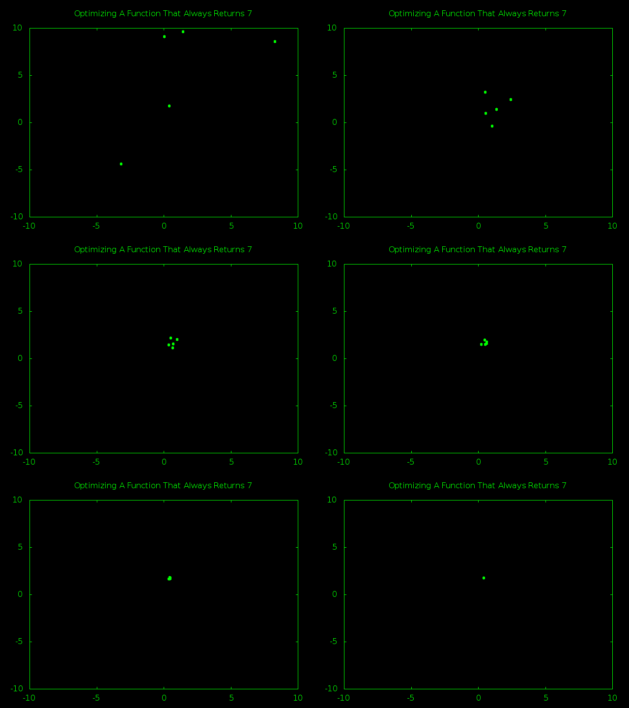
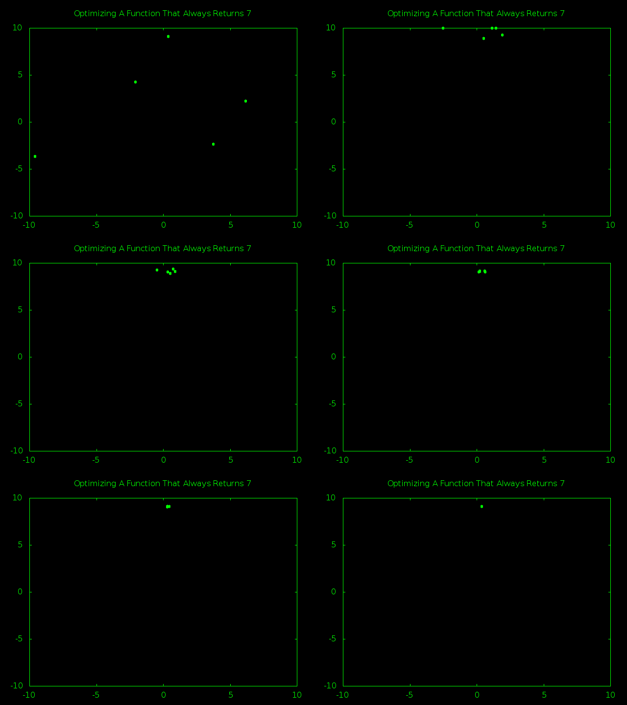
An animation of a swarm optimizing a flat function

A swarm optimizing a function with no optimum… whatever that means


Basically the swarm just latched onto the first guess it made, which obviously returned 7. Since no other guess ever returned anything smaller than 7 the swam quickly gravitated to that first, random guess.


You can see here that I ran the optimizer again and it got a different but equally correct answer. So the swarm optimizer can handle flat functions just fine by generating a random answer and sticking with it.


An animation of a swarm optimizing a flat function

Same size swarm optimizing the same flat function but getting a different random answer


That was actually more boring than the parabola. Let’s move onto something else.


There’s A Hole In Your Problem Space


The parabola is a nice smooth function where values change gradually and it is easy to just “roll down the hill” to find the minimum. We’re going to mix that up now by creating a function that is mostly a smooth parabola, but also has a sudden big hole somewhere around (3,3). The true minimum will be inside that hole.


(defun double-parabola-with-hole ( x y)
   (if (and (>= x 3) (<= x 3.1) (>= y 3) (<= y 3.1))
      (- (+ (* x x) (* y y)) 100)
      (+ (* x x) (* y y))))


This is a pretty simple step function. If X and Y are both inside the tiny window of 3 to 3.1 then we calculate the normal parabola and then subtract 100. Otherwise we just calculate the normal parabola. This results in a problem space that basically looks like a giant bowl with a really deep but tiny square hole cut into one of the sides.


The test here is to see if the swarm can find that hole or if it just rolls down the hill and gets stuck thinking (0, 0) is the the true minimum instead of the local minimum it really is.


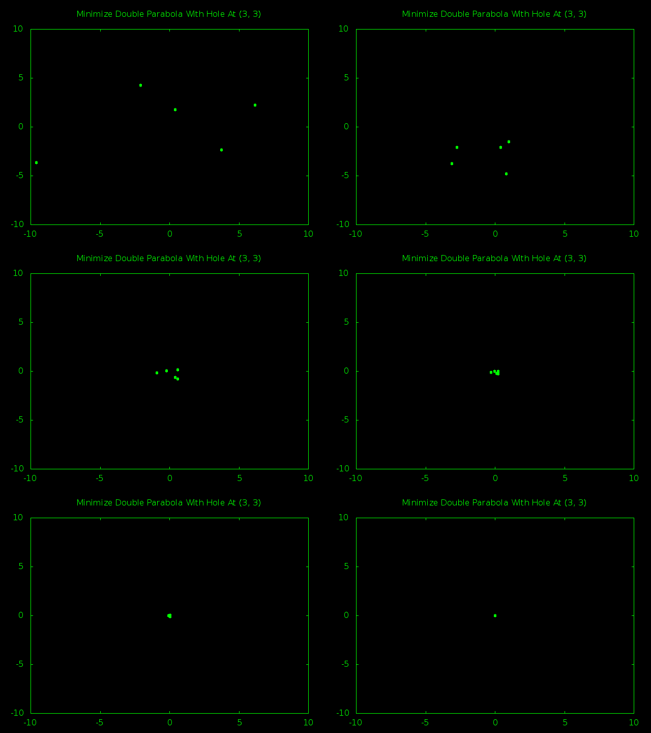
An animation of a small swarm failing to optimize an unusual function

That’s not the minimum!


A quick look at this animation shows that my normal 5 particle swarm running for 75 iterations just can’t find the tiny true minimum hiding at (3, 3).


Increasing the iteration count isn’t going to help; the swarm will just spend even more time zooming ever closer to the local minimum at (0, 0).


But if more time won’t help, what about more particles? The more particles we have zooming around the bigger the chances there are that one of them will eventually stumble across our hole and alert the swarm that they really need to be looking in the (3, 3) region.


So I started kicking up the size of the swarm. 50 particles was no good. 100 particles failed too. 200, 300, 400, 500… nothing. They all just gravitate to the origin.


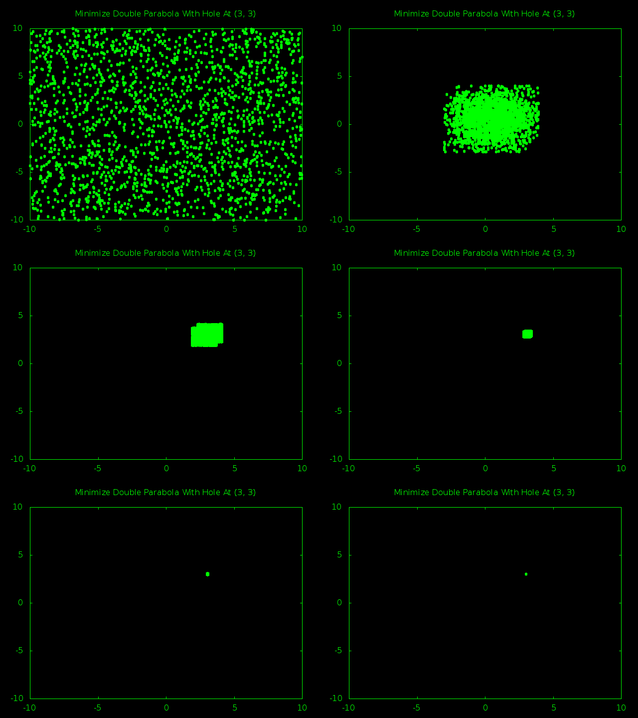
Time for the big guns. A 1,000 particle swarm managed to find the true minimum hole a little less than half the time. A 2,000 particle swarm had closer to an 80% success rate. Here is a snapshot of the 2,000 particle swarm in action.


bigswarmcanfindsmallhole


First off, isn’t it kind of cool how the way we define our borders wound up squashing the swarm into a big rectangle shape instead of the generic blob we would expect?


Second, you can actually see that at the start the swarm still thought that (0, 0) was the smartest place to look for a minimum. It was only after the first few steps that one of the particles got lucky and noticed that there were even smaller values around (3, 3) and managed the drag the entire swarm in the right direction.


I suspect that if our hole was even farther away from the obvious fake minimum then it would take even more particles to reliably find it. For example, if the hole was at (9, 9) you would probably needs tends of thousands of particles just to make sure that even after most of the particles headed straight for the origin there were still a few thousand slowly circling the edge.


Exercise for the reader: Create a double-parabola with a 0.1 x 0.1 hole at (9, 9). Find out how big the swarm has to be before it can find the right answer 90% of the time.


Bonus Exercise for the reader: Create a series of double parabolas with 0.1 x 0.1 holes at (1, 1), (2, 2), (3, 3), (4, 4) and so on until (9, 9). Record how big the swarm has to be in order to achieve 90% success rate for each hole. Is there a pattern between how far away the hole is from the natural parabola minimum and how large the swarm has to be to find it?


How To Get Better At Finding Holes


This whole “find the tiny square where the optimal value is hiding” shows off the big weakness of our overly simplistic swarm intelligence. Because particles obsess only about the global best answer so far they do not spend a lot of time exploring their own corner of problem space before shooting off and clumping up with the other particles. Unless we use a huge swarm we are at high risk of getting stuck on local optimums.


There are a couple ways an ambitious reader could fix this problem. One would be to upgrade the swarm so that particles keep a memory of their own best solution so far in addition to the global best solution and then have them choose their next guess based off of both of those numbers. This will slow down how fast the swarm clumps together and give you a better look at all of problem space.


Of course, this isn’t a miracle solution. It really only works in scenarios where you have multiple, obvious trends. Imagine a plane filled with lots of little valleys, some shallower than others. Local best answers allow particles to roll towards the bottom of their own valley before getting too excited about the global smallest answer so far. This way a particle that randomly starts out at the bottom of a shallow valley can’t dominate all the other particles that randomly started near the top of much deeper, and better, valleys.


However, think back to our parabola with a whole. All the particles are in the same “bowl”. Their local bests will lead them to roll down to the center, just like the global best did. So in this particular case the local best doesn’t really help us.


So another option might be to add some extra chaos into the system by creating a new type of “scout” particle that doesn’t care as much about global or local bests as a normal particle would. Instead it randomly changes its velocity, breaking away from the central swarm in order to explore areas that the rest of the swarm ignored.


To be honest it’s a long shot that one of these scout particles is going to find something that the rest of the swarm somehow didn’t on their way to clumping together… but a small chance is better than no chance. Even better, since scout particles don’t settle down like normal particles their chance of finding a new answer just keeps going up the longer the swarm is alive.


So if you plan on having a long running swarm, maybe on that runs forever and reports its current best every hour, then you really should probably code up some scout particles. This is especially important if you are working with a problem space that changes. It would be sad if a new optimum suddenly appeared in a corner and you never found out because your particles had already clumped together somewhere else and were no longer active enough to notice the change.


A Bumpy Problem Space


So we’ve already covered a problem with no optimums* and a problem with one very hard to find optimum. Now let’s try a problem with a couple dozen optimums spread evenly throughout problem space.


(defun double-sine-wave (x y)
   (+ (sin x) (sin y)))


I’m sure you’ve seen a sine wave. This is two sine waves put together in what would look like a giant field filled with dozens of hills and valleys, all exactly the same size.


Honestly this will be a boring experiment. If we had local minimum code then we could probably see a bunch of particles rolling around their nearest valley before finally all grouping up at some randomly selected global best valley… but that’s not what we have. All we have is a global minimum so odds are the particles will bounce around a bit and then all clump up at one spot pretty fast.


[5]> (defparameter *swarm-size* 25)

*SWARM-SIZE*

[6]> (defparameter *swarm-iterations* 75)

*SWARM-ITERATIONS*

[7]> (defparameter *swarm-output* (swarm-minimize-2d #’double-sine-wave ‘(-10 10) ‘(-10 10)))

*SWARM-OUTPUT*

[8]> (first *swarm-output* )

(-1.570653 4.7121253)

[9]> (double-sine-wave -1.57 4.71)

-1.9999969


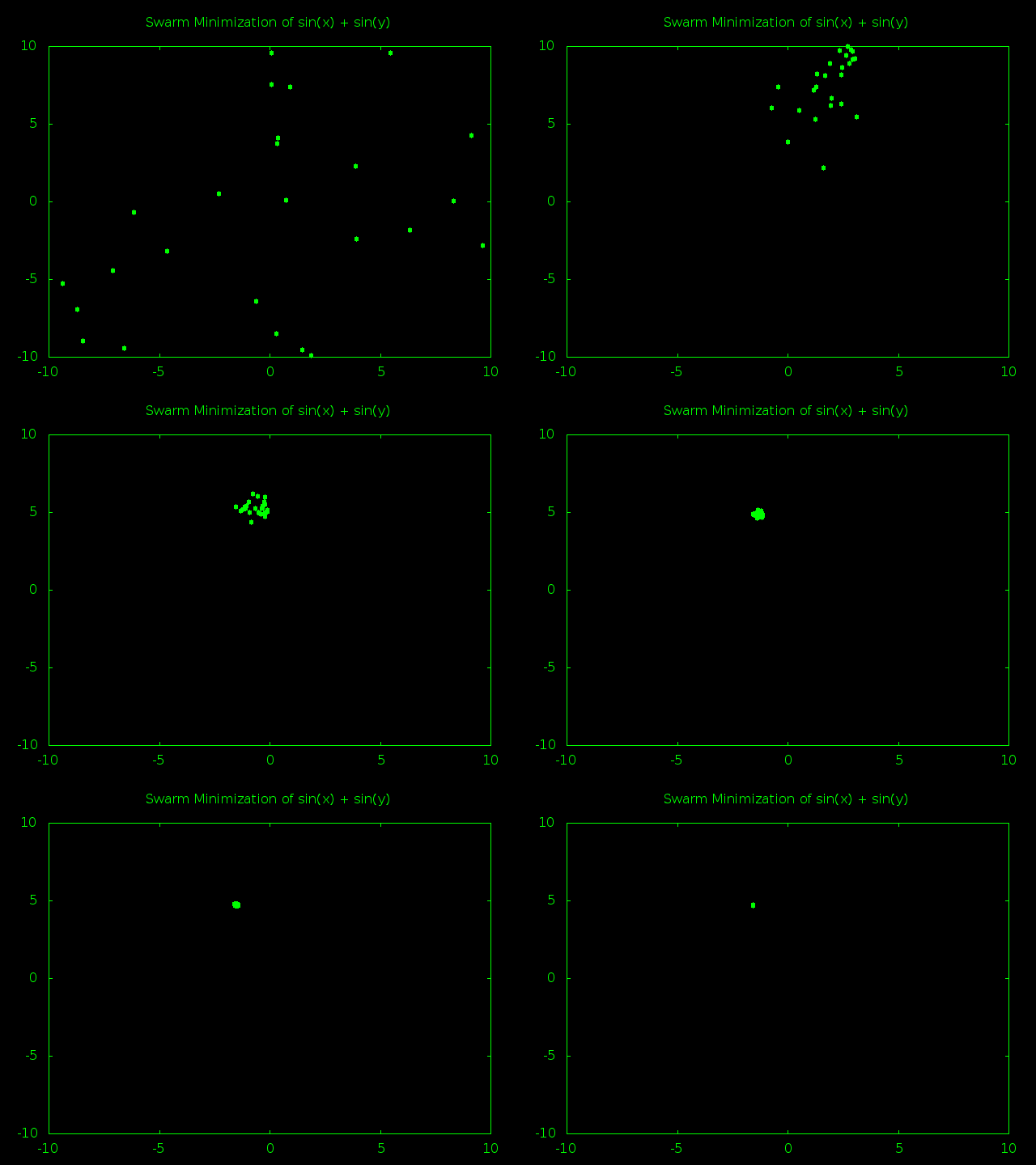
OK, -2 is the smallest value you can get by adding together two sine functions so good job there. Now it’s time to animate the history:


An animation of a swarm optimizing a sine wave based function

The minimum is over here… or is it over here? Wait, definitely here!


Meh, I guess this is *kind-of* interesting. You can see how the first global minimum was inside of one valley, then a particle bumped into another valley and the whole swarm started moving that way before bumping into a third valley and finally settling there. It’s at least more interesting than the standard double parabola where everything heads for the center almost from the very start.


Time To Transcend This Plane Of Existence


I think I’ve covered everything I wanted to for two dimensional swarms, so next time around we’ll be working on creating a more general swarm that can handle higher dimension equations. The hardest part is probably going to be coming up with some easy to understand test functions.


Does anybody have any idea what a nine dimensional octuple-parabola would look like?


* Or is that an infinite number of optimums? Consider it the math version of the “is the glass half empty or half full” question.