Let’s Program A Swarm Intelligence 11: Turning Your World Upside Down

Maxing Our Mins


Our current AI is pretty good at minimizing equations, but what if you want big numbers instead of small numbers? For example, what if you want to find the maximum for the equation -1 * (x^2 + y^2)? Or as we say in Lisp:


(defun inverse-double-parabola (x y)
   (* -1 (+ (* x x) (* y y))))


This is the opposite of our normal double parabola. This time the bigger x and y get the more negative and small our answer becomes. So the origin (x=0, y=0) will give us the biggest possible answer instead of the smallest possible answer.


a parabola and an inverse parabola

A badly drawn sketch of the difference between a parabola and an inverse parabola

Now how are we going to go about building a maximizer for this problem? Well, hopefully you remember back in part three where we showed that you can turn a minimizer into a maximizer just by multiplying all your results by -1 before passing them to the minimizer. That’s enough to turn big answers into small answers so our minimizer can track them down.


Our next task is clear then: We need to create a new function that accepts a maximizable function, creates an inverse version of it and then feeds that inverse function into the minimizer we already have.


Lambda: Kind Of A Big Deal


Since it looks like we need to build new functions on the fly I think it’s about time to introduce the mighty lambda. This powerful Lisp feature allows us to create new anonymous functions right on the spot and then immediately assign them to a variable or pass them to a function.


Explaining anonymous functions and how they differ from named functions can be a little tricky, so let’s just jump to some examples. The basic syntax is:


(lambda (argument names) (code that uses argument names here))


For example, here is a lambda function for multiplying a number by 3:


(lambda (x) (* 3 x))


And here it is an example of using lambda to assign an anonymous function to a variable and call it later:


[1]> (defparameter *test-fn* (lambda (x) (* 3 x)))

*TEST-FN*

[2]> (funcall *test-fn* 9)

27


For a second example let’s look at something from our swarm intelligence code. Here is how we normally minimize a double parabola, by passing a reference to a pre-existing doube-parabola function:


(swarm-minimize-2d #'double-parabola '(-10 10) '(-10 10))


But we could also use lambda to just define a double parabola function right on the spot:


(swarm-minimize-2d (lambda (x y) (+ (* x x) (* y y))) '(-10 10) '(-10 10))


This syntax is going to be very important in just a few seconds!


Lambda Maximizer To The Max!


Now we can talk about how to use Lisp to invert the results of a function call. First, I’m sure you remember that when we have a function inside of a variable named “fn” we can call that function and pass it two variables like this:


(funcall fn x y)


And if we know that the function is going to have numeric output we can invert it like this:


(* -1 (funcall fn x y))


Now here comes the tricky part. If we have a function inside a variable like “fn” we can use lambda to create a new function that accepts two variables, passes them to “fn” and then inverts the result. We can then pass this entire anonymous inverse function to swarm-minimize.


(defun swarm-maximize-2d (fn x-limits y-limits)
   (swarm-minimize-2d (lambda (x y) (* -1 (funcall fn x y))) x-limits y-limits))


If you understand this one-line function then you’ve mastered a lot of what makes Lisp so powerful.


And here it is in action:


[7]> (defparameter *swarm-iterations* 75)

*SWARM-ITERATIONS*

[8]> (defparameter *swarm-output* (swarm-maximize-2d #’inverse-double-parabola ‘(-10 10) ‘(-10 10)) )

*SWARM-OUTPUT*

[9]> (first *swarm-output*)

(-5.1605515E-5 -0.0015050085)


What do you know, that’s more or less the maximum for a double inverse parabola.


Stay On Target


Back in part three we also talked about how you could use a minimizer to help you hit a specific goal by minimizing the distance between your target and your results. We can pull this off as another one line function thanks to lambda:


(defun swarm-target-2d (fn target x-limits y-limits)
   (swarm-minimize-2d (lambda (x y) (abs (- target (funcall fn x y)))) x-limits y-limits))


[10]> (defparameter *swarm-output* (swarm-target-2d #’double-parabola 3 ‘(-10 10) ‘(-10 10)))

*SWARM-OUTPUT*

[11]> (first *swarm-output*)

(-1.5764234 -0.7178333)

[12]> (double-parabola -1.5764234 -0.7178333)

3.0003953


In this test I loaded up our classic double parabola and gave it a target of ‘3’. Seventy five iterations later the swarm comes up with (-1.6, -0.7) as a possible input and when we plug that in we get very close to the 3 we were hoping for. Success!


Conclusion


We covered one of the stranger but more powerful features of the Lisp programming language and used it to magically transform our particle swarm minimizer into a particle swarm maximizer and a particle swarm goal seeking machine. I’d say that’s a pretty good day’s work.


Join me next time as I take our three swarm optimization functions and then do everything in my power to stump them with hard to optimize inputs and strange function patterns.

Let’s Program A Swarm Intelligence 10: Let Me See…

Impress Your Friends And Family With Data Visualization!


We now have a working two dimensional particle swarm optimizer that can reliably minimize simple problems. That’s pretty cool, but you have to be a computer geek to really appreciate it. Give this program to a non computer geek and all they’ll see is a boring command line tool that spits out answers to obvious problems. They don’t understand all the nifty logic going on behind the scenes.


So why not show it to them?


Our swarm is made up of particles that each have a known x and y value. We can graph those points to show what kind of guesses the particles are making at any given point in time. Even people who don’t understand exactly what your program is doing will be impressed by a series of fancy graphs.


I mean, they *might* be impressed. You never know. You must have at least one friend that really likes graphs.


Enter the gnuplot


How to go about turning our swarm data into a swarm graph? Well, we could write our own custom Lisp code for graphing data… but why bother? There are tons of graphing programs already out there and the more time we spend on graphs the less time we have to spend on artificial intelligence. Life is about prioritization!


So what do we need in a graphing program? Honestly, just about any program that can read data from a file and produce scatter-plots from it is good enough for us. You could probably do it with an Excel macro, for example.


But since I’m on a Linux machine at the moment the most convenient option for me is a handy program called “gnuplot”. It’s a powerful graphing tool with tons and tons of options; way more than I could cover in a single blog post. But after messing around for a few hours I figured out some syntax to create one big file that can generate multiple graphs all at once. Perfect for printing out our entire swarm history all in one go!


It looks a little like this:


set terminal png x000000
set nokey
set border lc rgb "#00FF00"
set title "Swarm Minimization: x^2 + y^2" textcolor rgb "#00FF00"

set output 'plot0.png'
plot [-10:10] [-10:10] '-' using 1:2 pt 7 lc rgb "#00FF00"
0.3288231 9.875179
3.6807585 7.472683
-8.19067 -3.7102547
-1.549223 -8.636032
3.1139793 1.0444632
EOF
set output 'plot1.png'
plot [-10:10] [-10:10] '-' using 1:2 pt 7 lc rgb "#00FF00"
8.927804 -4.897444
-10 3.5666924
1.7747135 2.2790432
10 5.109022
10 5.0106025
EOF


The first four lines set up some generic style rules for our graphs. I start by setting the default graph to be an all black PNG image. I then turn off the automatic legend and set the line color (lc) of the graph border to be bright green (since the default black won’t show up against a black background). Finally I add a big green title to the top of the graph.


After that I pick out a name for the file where I want to save the first graph by using set output. Then I use the plot command to actually make the graph, which gets a little complicated.


The first two inputs to plot are the x and y boundaries we want to use in our graph. The third argument is the location of the data we want to graph. Normally this would be a filename, but ‘-‘ using 1:2 lets us instead just type the data we want right into the same file. After that we use pt 7 to choose how we want to draw our data points (7 is code for a filled circle) and use lc again to make our points just as green as our boundaries and title.


With all that out of the way we can finally include the data we want to graph. Each point is represented by two numbers, on their own line and with a space between them. After typing in all the numbers we use EOF to indicate that’s the end of our fake little inline data file.


Then we choose a filename for our next graph with another set output, repeat the plot command and then include the next set of data. And we do that again and again until we’ve graphed all the graphs we want graph.


Formatting Data


With that example file to work with we can start working on some Lisp to grab our swarm history and rearrange it into a gnuplot input file.


The first obstacle we have to deal with is the fact that our swarm intelligence stores history as a list of particle histories. This makes it very easy to grab and read the complete history of any individual particle. Unfortunately, when it comes to graphing we want to do the opposite. Instead of the complete history of one particle we want a single step in the history of every particle.


Example: If we want to draw a graph of how the swarm looked during its third loop through our algorithm we would need the third entry in the history list for every single particle. If we wanted to draw the swam during it’s sixth loop we would need the sixth entry in the history list of every single particle.


Fortunately this isn’t hard thank to loop (again!) and the handy nth function. Like you might expect, the nth function lets you grab items from anywhere inside a list.


(defun get-swarm-history-step-n-2d (swarm-history step)
   (loop for history in swarm-history
      collect (nth step history)))


These three lines of code are all that we need to get a snapshot of the entire swarm at any point in its history.


Efficiency Warning


One quick note here for all you efficiency buffs out there. Lisp lists are wonderful and flexible data structures but they aren’t always the fastest.


The main problem is that you can’t just grab random items out of a list, you have to visit them in order. To get to the third item in a list you first have to grab the first item. The first item tells you the location of the second item, and then the second item helps you find the third item. Now if you instead wanted to find the one millionth item in a list… well you can see how that could start to be a waste of time.


For small amounts of data this isn’t a problem. But when you really need fast access to data no matter where it is inside a list you would probably be better off with something that does allow random access, like an array. Which Lisp supports. So if you want to slightly boost the speed of your swarm that’s one change you could make.


Printing The Data


Now that we can grab slices of swarm history we can put together one last big function to take one slice from every step in the swarm’s history and glue them all together into a file for gnuplot.


(defun print-swarm-history-graph-file-2d (filename swarm-history title x-bounds y-bounds)
   (with-open-file (stream filename :direction :output)
      (format stream "set terminal png x000000~%")
      (format stream "set nokey~%")
      (format stream "set border lc rgb \"#00FF00\"~%")
      (format stream "set title \"~a\" textcolor rgb \"#00FF00\"~%~%" title)
      (loop for i from 0 to (1- (length (first swarm-history))) do
         (format stream 
            "set output 'plot~a.png'~%plot [~a:~a] [~a:~a] '-' using 1:2 pt 7 lc rgb \"#00FF00\"~%"
            i (first x-bounds) (second x-bounds) (first y-bounds) (second y-bounds))
         (loop for position in (get-swarm-history-step-n-2d swarm-history i) do
            (format stream "~a ~a~%" (first position) (second position)))
            (format stream "EOF~%"))))


It’s a big looking function but most of that is just calls to format. Look at this function alongside the sample gnuplot file and it’s pretty easy to see what is going on.


One complication worth looking at is with-open-file. It let’s us create or open a file and then read or write data to it. In this particle case we use with-open-file to create a handle named “stream” pointing to whatever filename is stored in our filename variable. Then we can use (format stream “some text”) to send text to a file instead of to the screen.


And with that the rest of the function is pretty straight forward. We start out by printing all the special rules we determined we need at the beginning of every gnuplot file.


After that we can print the specific coordinates for each step with two nested loops. The first loop needs to run once for every step in our history and set. Then for each step the inner loop needs to get all the individual particle coordinates for that step and add them to the file.


The Moment You’ve All Been Waiting For…


[30]> (load “swarm.lisp”)

;; Loading file swarm.lisp …

;; Loaded file swarm.lisp

T

[31]> (defparameter *swarm-size* 25)

*SWARM-SIZE*

[32]> (defparameter *swarm-iterations* 70)

*SWARM-ITERATIONS*

[33]> (defparameter *swarm-output* (swarm-minimize-2d #’double-parabola ‘(-10 10) ‘(-10 10)))

*SWARM-OUTPUT*

[34]> (first *swarm-output*)

(-1.5024608E-4 0.0011557455)

[35]> (defparameter *swarm-history* (second *swarm-output*))

*SWARM-HISTORY*

[36]> (print-swarm-history-graph-file-2d “swarm-history.txt” *swarm-history* “Swarm Minimization: x^2 + y^2” ‘(-10 10) ‘(-10 10))

NIL


That produces a “swarm-history.txt” file that we can feed into gnuplot. Although I personally suggest you move it to a new folder first before running it. Generating dozens or hundreds of graphs all at once can make a real mess of your development folder. I did all my graph work in a folder named “output” to keep it separate from my code files.


Wherever you decide to do your work, generating your graphs is as easy as:


gnuplot swarm-history.txt


And now you have one PNG file for every guess your swarm AI made. You can finally see the code working.


The Really Cool Part


Now that we have a graph of every step in our swarm algorithm the only logical thing to do is string them all together into one big animation: a simple enough trick for a graphic manipulation tool like Gimp. I’ll leave it up to you to find a good tutorial on how that works.


Now we can finally see exactly what our swarm has been up to, and it was just what we expected.


An animated graph of a particle swarm optimizer

Look At That Swarm Swarming!


The swarm starts out spread out randomly all over problem space and the particles are moving very fast, bouncing around at high speeds and trying tons of different answers. After just a few rounds of guesses the particles start to gravitate towards (0,0), the true best answer of x^2 + y^2. As time goes on the particles start slowing down so they can better examine the promising answers near the center of the graph. Finally all the particles converge and stick to one best answer, or at least really close to it.


Next: More Data To Visualize


We now have all the tools we need to visually demonstrate the inner workings of our swarm intelligence (which is a great way to show off to friends). Next time we’ll put those tools to good use by thinking up some new equations for our swarm to optimize. We’ll also finally get around to improving our optimizer to maximize and search for target values instead of just minimizing.

Let’s Program A Swarm Intelligence 9: All Together Now

We’re Already Past The Hard Part


Like I’ve told you again and again a particle swarm optimizer is just a bunch of particles/numbers moving around and making guesses at how to optimize a problem until we feel like we’re reasonable close to the ‘true’ best answer to our problem.


Last time we wrote some code for moving one particle around, so now all we need is some code for moving lots of particles around. We can actually do this with just two loops: One big outer loop that keeps repeating until we have our final answer and a smaller inner loop that updates every particle in the swarm once for each step through the main loop.


With that in mind there are really only two questions left to answer: How big should our swarm be and how do we decide when we are done looking for better answers?


The simplest solution to both problems is to hard code some values. We will choose a specific number of particles for our swarm and we will also choose how many times we want the swarm to update those particles before deciding on a final answer.


This obviously isn’t the only, or best, way to do this. It might be smarter to decide when to stop by keeping track of how long it’s been since we’ve found a better answer. If we haven’t found on after a few dozen or hundred updates then we stop. This way we can leave it up to the swarm to decide when it is done and we don’t have to worry so much about accidentally cutting the swarm off while it’s still doing good work.


But that can get complicated. So for now let’s just stick with hard coding some values. Just pop them in some global variables so we can easily adjust them for each problem we try. We’ll keep our default values really small so it’s easy to debug:


(defparameter *swarm-size-2d* 5)
(defparameter *swarm-iterations* 5)


Now we just need to build a swarm of size *swarm-size* and loop through it *swarm-iterations* times. The update-swarm-particle-2d code from last post will do the rest of the work for us:


(defun swarm-minimize-2d (fn x-limits y-limits)
   "A particle swarm optimizer for two dimensional equations"
   (let ((swarm   (generate-swarm-2d *swarm-size*
                     (first x-limits) (second x-limits)
                     (first y-limits) (second y-limits))))
      (loop for i from 1 to *swarm-iterations* do
         (loop for particle in (particle-list swarm)
            do (update-swarm-particle-2d particle swarm fn x-limits y-limits)))
      (list (best-x swarm) (best-y swarm))))


Go Forth and Optimize, My Swarmy Minions!


That’s all our swarm needs in order to start solving problems, so let’s give it a spin. We’ll be feeding it our handy double-parabola test function and seeing how close it comes to the real answer. Remember that the true minimal optimum for a double parabola is (0, 0):


[34]> (swarm-minimize-2d #’double-parabola ‘(-10 10) ‘(-10 10))

(-2.5209198 3.1263676)


Ok… not so great. Kind of disappointing, actually.


But wait! We only had five particles making five guesses each. Of course they couldn’t find a good answer. Let’s give them a little more time to work and see if that improves anything:


[35]> (defparameter *swarm-iterations* 100)

*SWARM-ITERATIONS*

[36]> (swarm-minimize-2d #’double-parabola ‘(-10 10) ‘(-10 10))

(2.5831852E-5 -6.708622E-6)


Much much better! Almost perfect, in fact. We’re within a rounding error of (0,0). Our swarm intelligence has successfully done something intelligent! Congratulations, an AI programmer is you!


Record Keeping


Getting good answers is pretty cool, but back in the design phase we decided that we were also interested in seeing the path our particles took in order to find that answer. That’s why all of our particles have that “history” data slot. You remember, that one that we had to write that weird nested list append thing to keep updated.


Because every particle keeps track of its own history generating a swarm-wide history is as easy as running through the swarm’s particle list and gather up all the individual histories into one big list. Which is yet another problem that the loop macro can solve for us. Honestly I probably could have titled this series “Let’s Use The Loop Macro To Solve All Our Problems”.


Anyways, here’s a function for building a swarm history and here’s an updated swarm-optimizer that includes that history in it’s output:


(defun get-swarm-history-2d (swarm)
   (loop for particle in (particle-list swarm)
     collect (history particle)))


(defun swarm-minimize-2d (fn x-limits y-limits)
   "A particle swarm optimizer for two dimensional equations"
   (let ((swarm (generate-swarm-2d *swarm-size*
                   (first x-limits) (second x-limits)
                   (first y-limits) (second y-limits))))
      (loop for i from 1 to *swarm-iterations* do
         (loop for particle in (particle-list swarm)
            do (update-swarm-particle-2d particle swarm fn x-limits y-limits)))
      (list (list (best-x swarm) (best-y swarm)) (get-swarm-history-2d swarm))))


Now Let’s shrink our swarm size and our number of guesses back down and give the new code a test run.


[39]> (defparameter *swarm-size* 2)

*SWARM-SIZE*

[40]> (defparameter *swarm-iterations* 4)

*SWARM-ITERATIONS*

[41]> (swarm-minimize-2d #’double-parabola ‘(-10 10) ‘(-10 10))

((-0.11861801 -0.97045755)

(((8.618713 -8.651136) (10 -0.23300552) (10 6.501499) (8.640749 9.647516))

((-8.614849 -7.199463) (-0.11861801 -0.97045755) (6.678367 4.012747)

(10 6.5043488))))


That’s a lot of parenthesis to read through but I bet you can see what happened. The first pair of numbers drowning in those parenthesis is the best answer the swarm has found so far (which is pretty bad since we only ran the algorithm through four steps). After that you might be able to make out that the remaining pairs of numbers are split into two lists of four. Those are the histories of the paths our two particles took through their four step journey.


And with that our two dimensional particle swarm optimizer is done. It runs the algorithm, finds the answers and spits back all the data we wanted from it.


Complete 2D Particle Swarm Optimizer Code


Now that this part of our project is “done” I imagine you’ll be wanting another full code dump. I keep all the following code in a file called “swarm.lisp”:


;Helper Functions
(defun ranged-random (min max)
    (+ min (random (float (- max min)))))

;Particle Related Code
(defclass particle-2d ()
    ((x-coord
        :initarg :x-coord
        :accessor x-coord)
    (y-coord
        :initarg :y-coord
        :accessor y-coord)
    (x-vel
        :initarg :x-vel
        :accessor x-vel)
    (y-vel
        :initarg :y-vel
        :accessor y-vel)
    (history
        :accessor history
        :initform () )))

(defun generate-particle-2d (x-min x-max y-min y-max)
    (let ((x-range (- x-max x-min))
          (y-range (- y-max y-min)))
      (make-instance 'particle-2d
          :x-coord (ranged-random x-min x-max)
          :y-coord (ranged-random y-min y-max)
          :x-vel (ranged-random (- x-range) x-range)
          :y-vel (ranged-random (- y-range) y-range))))

(defun print-particle-2d (particle)
    (format t "x:~a~%y:~a~%x-vel:~a~%y-vel:~a"
        (x-coord particle)
        (y-coord particle)
        (x-vel particle)
        (y-vel particle)))

(defun one-line-print-particle-2d (particle)
    (format t "pos:<~a, ~a> vel:<~a, ~a>~%"
        (x-coord particle)
        (y-coord particle)
        (x-vel particle)
        (y-vel particle)))

;Swarm Related Code
(defclass swarm-2d ()
    ((best-x
      :initarg :best-x
      :accessor best-x
      :initform 0)
     (best-y
      :initarg :best-y
      :accessor best-y
      :initform 0)
     (best-answer
      :initarg :best-answer
      :accessor best-answer
      :initform most-positive-long-float)
     (particle-list
      :accessor particle-list)))

(defun generate-swarm-2d (particle-count x-min x-max y-min y-max)
    (let ((new-swarm (make-instance 'swarm-2d)))
      (setf (particle-list new-swarm) 
            (loop for i from 1 to particle-count 
               collect (generate-particle-2d x-min x-max y-min y-max)))
      new-swarm))

(defun print-swarm-2d (swarm)
    (format t "Best input:<~a, ~a>~%Best answer:~a~%"
        (best-x swarm)
        (best-y swarm)
        (best-answer swarm))
    (loop for particle in (particle-list swarm)
       do (one-line-print-particle-2d particle)))

;Swarm Optimization Code
(defparameter *swarm-size* 5)
(defparameter *swarm-iterations* 5)

(defun swarm-minimize-2d (fn x-limits y-limits)
   "A particle swarm optimizer for two dimensional equations"
   (let ((swarm (generate-swarm-2d *swarm-size*
                      (first x-limits) (second x-limits) 
                      (first y-limits) (second y-limits))))
       (loop for i from 1 to *swarm-iterations* do
        (loop for particle in (particle-list swarm)
           do (update-swarm-particle-2d particle swarm fn x-limits y-limits)))
           (list (list (best-x swarm) (best-y swarm)) (get-swarm-history-2d swarm))))

(defun update-swarm-particle-2d (particle swarm fn x-bounds y-bounds)
    (update-particle-history-2d particle)
    (let ((particle-answer (funcall fn (x-coord particle) (y-coord particle))))
        (when (< particle-answer (best-answer swarm))
            (setf (best-answer swarm) particle-answer)
            (setf (best-x swarm) (x-coord particle))
            (setf (best-y swarm) (y-coord particle))))
    (update-particle-velocity-2d particle (best-x swarm) (best-y swarm))
    (let ((updated-x (+ (x-coord particle) (x-vel particle)))
           (updated-y (+ (y-coord particle) (y-vel particle))))
       (setf (x-coord particle) (max (first x-bounds) (min (second x-bounds) updated-x)))
       (setf (y-coord particle) (max (first y-bounds) (min (second y-bounds) updated-y)))))

(defun update-particle-history-2d (particle)
    (setf 
      (history particle) 
      (append 
         (history particle) 
         (list (list (x-coord particle) (y-coord particle))))))

(defparameter *original-velocity-weight-2d* 0.8)
(defparameter *target-velocity-weight-2d* 0.3)

(defun update-particle-velocity-2d (particle target-x target-y)
    (let ((target-x-vel (- target-x (x-coord particle)))
          (target-y-vel (- target-y (y-coord particle))))
       (setf (x-vel particle) 
             (+ (* *target-velocity-weight-2d* target-x-vel) 
                (* *original-velocity-weight-2d* (x-vel particle))))
       (setf (y-vel particle) 
             (+ (* *target-velocity-weight-2d* target-y-vel) 
                (* *original-velocity-weight-2d* (y-vel particle))))))

(defun get-swarm-history-2d (swarm)
    (loop for particle in (particle-list swarm)
        collect (history particle)))

;Functions To Optimize
(defun double-parabola (x y)
    (+ (* x x) (* y y)))


More Done Than Done


With the 2D swarm finished you might think our next goal is to tackle the general swarm intelligence project, but I’m not quite ready to move beyond the second dimension just yet. I’d like to run a few more tests and play with some data first. So join me next time as we take a look at the wonderful world of data visualization!

Let’s Program A Swarm Intelligence 8: It Lives!

An Extremely Easy Sample Optimization


Now that we have a swarm it’s time to teach it how to go out and conquer the stars… I mean teach it how to properly optimize a function. And for that we’re going to need a test function we can practice with.


We want our first testing function to be simple enough that we humans can double check the computer’s work without having to waste thirty minutes pecking numbers into our graphing calculators*. Later on we can come up with some complex tests to really give the swarm a run for its money but for now we want easy.


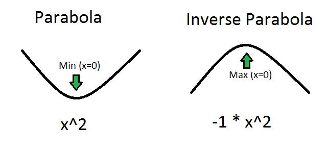
And what’s easier than a parabola? You just can’t beat good old x^2 when it comes to predictable equations with an obvious minimum. Everyone can see that the obvious minimum of x^2 is when x equals 0, right?


But this is a two dimensional swarm, and parabolas are only single variable problems. We want a two dimensional problem. So behold! The double parabola: x^2 + y^2


The optimized minimum of this two variable problem is just as obvious as the one variable version. When both x and y are 0 the final answer is also zero.


In Lisp terms our double parabola looks like this


(defun double-parabola (x y)
   (+ (* x x) (* y y)))


If we feed this function into our particle swarm it should ideally spit back an answer very close to (0, 0). And now that we know what we’re looking for we can start programming some swarm logic.


A Reminder Of How This Whole Thing Works


You’re probably getting bored of me explaining the basics of swarm intelligence over and over again, but if years of Sesame Street have taught me anything it’s that repetition is an important part of learning. So here we go, one last time, to make sure you’re 100% ready to actually program this thing.


Our goal is to take an equation with two variables and try to find the input that will give us the most optimal answer, defined here as the smallest answer possible (a minimum). So if we find two possible answers of 10 and 5 we consider the smaller number, 5, to be more optimal.


In order to try and find the most optimal, minimal answer for the entire equation we create a bunch of particles that all have a position and a velocity. The position represents a possible set of input values to the equation. The velocity represents how much we want to increase or decrease those inputs before making our next guess.


We run the swarm by looping through all the particles and feeding their position/input into the function we are trying to optimize. We keep track of what input has produced the most optimal guess so far. After each particle has made it’s guess we update their velocity to point a little bit more towards our best answer. Then we move all the particles based off of their velocity and repeat the process.


What this should do is create a bunch of random particles that make tons of random guesses. As time goes on the particles will start agreeing on a best answer and their velocity will begin to point towards it. This will cause the particles to get closer to each other so they can focus their guessing power around good answers. Eventually the particles will all be clumped together and stop finding new, better answers. At that point we grab the best answer so far and call it our best educated guess on what the true minimum must be.


Starting Small


This is a pretty complex problem, or at least pretty complex for a single blog post. So instead of jumping straight in and trying to write an algorithm for updating an entire swarm let’s take it easy and write an algorithm for updating a single particle. We’ll need that function for the bigger swarm algorithm anyways.


Updating a particle is a five step process:

  1. Add the particle’s current position to its history.
  2. Use the particle’s current position to generate an answer to the function we want to optimize.
  3. Compare that answer to the current swarm best answer. If it is better, update the swarm best.
  4. Update the particle’s velocity to point slightly more towards the swarm best.
  5. Update the particle’s position based off of it’s velocity, but make sure it stays in the bounds of the problem.


In order to pull all that off we’re going to need the following pieces of information:

  1. The particle we are updating
  2. The swarm we are updating
  3. The function we are optimizing
  4. The boundaries of the problem.


Which leads us to this:


(defun update-swarm-particle-2d (particle swarm fn x-bounds y-bounds)
   ;Code goes here)


Turning A Function Variable Back Into A Function


One more bit of Lisp you’re going to need to know in order to construct this algorithm. You might remember that Lisp lets you create a function reference really easy with the #’function-name syntax, which will make it easy for us to toss our double-parabola around as #’double-parabola. But putting a function into a variable is only half the battle. We also need to get it back out.


This is as easy as using funcal. The first argument is a variable holding a function reference and then the rest of the arguments become data for that function. Ex:


[4]> (defparameter *test-fn* #’double-parabola)

*TEST-FN*

[5]> (funcall *test-fn* 2 5)

29


Would You Like To Save Your Data?


With that out of the way we can start going through the five steps of the algorithm. The first is to add the particle’s current position to its history, which is easy enough to do with the append function. This may not be the most efficient way to build the history data structure, but until we have real data on whether the algorithm is fast or slow there’s no point obsessing about this.


The trick to watch out for here is that append expects two lists. It then takes every item in the second list and puts it into a copy of the first list. So if we want to add a two item list to our history we can’t just pass the two item list; append will take it apart and put in the individual pieces. Instead we need to pass a list holding our two item list. append will take apart the outer list and leave the inner list alone.


(defun update-swarm-particle-2d (particle swarm fn x-bounds y-bounds)
   (setf
      (history particle)
      (append
         (history particle)
         (list (list (x-coord particle) (y-coord particle))))))


But that’s very ugly and takes up a lot of room. Let’s hide it in a function:


(defun update-swarm-particle-2d (particle swarm fn x-bounds y-bounds)
   (update-particle-history-2d particle))

(defun update-particle-history-2d (particle)
   (setf
      (history particle)
      (append
         (history particle)
         (list (list (x-coord particle) (y-coord particle))))))


Is That Your Final Answer?


With that little bit of record keeping code out of the way we can move on to the most important part of this entire algorithm: Checking whether or not the particle has a good answer in it. That’s the whole reason we programmed this swarm in the first place. The whole purpose of a particle is to test out new answers to see if they are better than the answer we’re currently using.


I can’t stress this enough! This is where the magic happens!


But just because it is important doesn’t mean it is hard. In fact, checking for answers is downright easy:


(defun update-swarm-particle-2d (particle swarm fn x-bounds y-bounds)
   (update-particle-history-2d particle)
   (let ((particle-answer (funcall fn (x-coord particle) (y-coord particle))))
      (when (< particle-answer (best-answer swarm))
         (setf (best-answer swarm) particle-answer)
         (setf (best-x swarm) (x-coord particle))
         (setf (best-y swarm) (y-coord particle)))))


We use funcall to feed the particle’s current x and y coordinates into whatever function has been passed into our optimizer. We store the answer in the local “particle-answer” variable and then compare it to the swarm’s current best answer. If the particle-answer is better we update the swam with a new best answer and new best coordinates. Pretty straightforward even with all the parenthesis.


A Little More To The Left…


We’re now halfway through our five item checklist for updating a particle. The next step is to adjust the particle’s velocity to point it slightly more towards our current best answer. There are lots of ways to do this, but for this Let’s Program I’m going to keep things really simple. This might make our swarm intelligence a little dumber than some of the more elegant algorithms, but it will make it much easier to blog about. If you’re interested in better swarms you can always use my code as a simple starting point to teach you enough of the basics to research and build your own, better optimizer.


For our simple velocity update what we want to do is calculate a target velocity that will send us hurtling straight towards the current swarm best answer. Then we want to take some fraction of that target velocity and add it to some fraction of the particle’s current velocity. Maybe something like 30% of the target velocity plus 80% of the current velocity (The two percentages don’t have to add up to 100%. We’re taking two fractions of two different things, not slicing one big thing into two pieces).


Deciding on exactly how much of each velocity to use has a big impact on your swarm. Large amounts of target velocity will focus your particles like a laser on whatever answer seems good at the time. Put more weight on current velocity and particles will lazily drift about exploring more data for a while before finally meeting up in the general vicinity of a good answer.


This is the sort of code that can get messy fast, so let’s put it into a function to avoid cluttering up update-swarm-particle-2d. All this function really needs to function is a particle to update and a target coordinate to point the particle at.


(defun update-swarm-particle-2d (particle swarm fn x-bounds y-bounds)
   (update-particle-history-2d particle)
   (let ((particle-answer (funcall fn (x-coord particle) (y-coord particle))))
      (when (< particle-answer (best-answer swarm))
         (setf (best-answer swarm) particle-answer)
         (setf (best-x swarm) (x-coord particle))
         (setf (best-y swarm) (y-coord particle))))
   (update-particle-velocity-2d particle (bext-x swarm) (best-y swarm)))


And now for the code itself:


(defun update-particle-velocity-2d (particle target-x target-y)
   (let ((target-x-vel (- target-x (x-coord particle)))
         (target-y-vel (- target-y (y-coord particle))))
      (setf (x-vel particle) (+ (* 0.3 target-x-vel) (* 0.8 (x-vel particle))))
      (setf (y-vel particle) (+ (* 0.3 target-y-vel) (* 0.8 (y-vel particle))))))


We figure out what the target x and y velocities should be by subtracting where we are from where we want to be, which will give us the speed we need to move at to hit our target in just one move. Example: The particle’s x position is five and the current best x is at two. Subtracting five from two gives us negative three (2-5=-3). So in order to reach the best x answer our particle needs to have a velocity of negative three units per update. Come up with a few more examples on your own if you’re having trouble following along.


Once we have target velocities it’s very easy to update the particle to a mix of 80% of it’s current velocity plus 30% of the best-answer seeking target velocity. Of course, it doesn’t have to be 80% and 30%. That’s just an example. We’ll probably have to run several tests to get a good feel for what values we should use. Let’s make that easier on ourselves by moving these magic numbers out of the code and into global variables.


(defparameter *original-velocity-weight-2d* 0.8)
(defparameter *target-velocity-weight-2d* 0.3)

(defun update-particle-velocity-2d (particle target-x target-y)
   (let ((target-x-vel (- target-x (x-coord particle)))
         (target-y-vel (- target-y (y-coord particle))))
      (setf (x-vel particle)
            (+ (* *target-velocity-weight-2d* target-x-vel)
               (* *original-velocity-weight-2d* (x-vel particle))))
       (setf (y-vel particle)
             (+ (* *target-velocity-weight-2d* target-y-vel)
                (* *original-velocity-weight-2d* (y-vel particle))))))


Much better.


But It Does Move!


Now that we’ve set the particle’s new velocity all that is left is to use that velocity to make the particle actually move. This is as simple as some basic addition and a couple quick checks to make sure the particles are in bounds.


(defun update-swarm-particle-2d (particle swarm fn x-bounds y-bounds)
    (update-particle-history-2d particle)
    (let ((particle-answer (funcall fn (x-coord particle) (y-coord particle))))
        (when (< particle-answer (best-answer swarm))
            (setf (best-answer swarm) particle-answer)
            (setf (best-x swarm) (x-coord particle))
            (setf (best-y swarm) (y-coord particle))))
    (update-particle-velocity-2d particle (best-x swarm) (best-y swarm))
    (let ((updated-x (+ (x-coord particle) (x-vel particle)))
           (updated-y (+ (y-coord particle) (y-vel particle))))
       (setf (x-coord particle) (max (first x-bounds) (min (second x-bounds) updated-x)))
       (setf (y-coord particle) (max (first y-bounds) (min (second y-bounds) updated-y)))))


I’m using a pretty cool trick here for keeping a number inside of bounds. Normally you would use two if statements to check if the number was bigger than the upper boundary or smaller than the lower boundary. Instead I keep it inside the upper boundary by just asking for the min value between our upper boundary and our given value. If our value is bigger than the upper boundary it will get discarded by the min. Then I do the same thing for the lower boundary with the max value. It lets you do boundary math in a single line of nested functions instead of needing conditional logic.


Not really a huge time saver, but I’ve always thought it was a nifty little pattern.


I Sure Hope This Works


Supposedly our code can now set particle history, update the swarm, change velocity and then move the particle. Time to see whether or not any of this code actually works, or if I’ll need to rewrite most of this before posting!


[1]> (load “swarm.lisp”)

;; Loading file swarm.lisp …

;; Loaded file swarm.lisp

T

[2]> (defparameter *test-swarm* (generate-swarm-2d 1 -10 10 -10 10))

*TEST-SWARM*

[3]> (defparameter *test-particle* (first (particle-list *test-swarm*)))

*TEST-PARTICLE*

[4]> (print-swarm-2d *test-swarm*)

Best input:<0, 0>

Best answer:8.8080652584198167656L646456992

pos:<0.40933418, -5.2009716> vel:<-6.6420603, -5.447151>

NIL

[5]> (update-swarm-particle-2d *test-particle* *test-swarm* #’double-parabola ‘(-10 10) ‘(-10 10))

-9.558693

[6]> (print-swarm-2d *test-swarm*)

Best input:<0.40933418, -5.2009716>

Best answer:27.21766

pos:<-4.904314, -9.558693> vel:<-5.313648, -4.357721>

NIL


Looks good. We build a swarm with exactly one particle and update that particle. You can see that before the update the swarm’s best answer is our ridiculously huge default. After the update the swarm’s best input has changed to the original position of the particle. We can also see that the particle’s velocity has shifted and that it updated it’s position successfully.


One Small Step For A Particle, Next A Giant Leap For Our Swarm


There was some pretty heavy code in this update, but that was expected. Updating particles is the heart of our entire algorithm. Now that that’s working the next post should be a breeze. All we have to do is upgrade from updating one particle once to updating an entire swarm of particles constantly… or at least until we get a workable answer.


* You’re reading an AI programming blog, of course you own a graphing calculator.

Let’s Program A Swarm Intelligence 7: Satisfying My OCD

You’re Calling THAT Good Code!?


Last time we wrote a bunch of functions for randomly generating particle swarms. But it was very messy and verbose and filled with way too many calls to slot-value.


Now this isn’t a huge problem. The code works and having to type a few hundred extra ‘slot-value’ characters per program only wastes a few minutes of our life. From a time efficiency perspective cute cat videos are a much bigger risk to your productivity than wordy code.


But wordy, messy code has other downsides. More code means more places for bugs to hide and lets you fit less code on the screen at one time. Less code on the screen means lots of scrolling and lots of short-term memory abuse. It gets annoying fast.


So whenever possible we want to write clean, compact code that let’s us see multiple functions on one screen and leaves bugs with nowhere to hide.


Building Objects Using initargs Instead Of setf And slot-value


Remember our code for putting together a random particle? It was absolutely filled with repetitive calls to (setf (slot-value someobject someslot) somevalue). All those nearly identical lines are more than enough to make my head spin and my eyes grow all blurry.


So let’s get rid of them by using some of the extra features of the Lisp object system.


Remember that the last argument in defclass is a list of the data slots we want inside our object. Up until now we were just using simple names but we can give our classes an extra boost by wrapping those names into a list and gluing some extra keywords to them. Basically instead of just saying “I want an x-coord slot” we’re going to be saying “I want an x-coord slot with these special features”.


One of the more useful keywords is :initarg (don’t forget the colon, that’s Lisp keyword naming convention). :initarg let’s you create a new keyword that can be used inside of make-instance to assign a value to a data slot as soon as it is created without having to make a separate call to setf. You can name this new keyword whatever you want but it’s traditional to just name it after the data slot it’s linked to, but with a keyword colon glued to it.


It’s really easier to show you than to try and explain it:


(defclass particle-2d ()
   ((x-coord :initarg :x-coord )
    (y-coord :initarg :y-coord )
    (x-vel :initarg :x-vel )
    (y-vel :initarg :y-vel )
    history ))


As you can see I’ve replace our old list of data slot names with three item lists including, in order, the name of the data slot, the :initarg keyword and the new keyword I want to use in make-instance. This let’s me create a new particle with one or more data slot already filled in like this:


(make-instance 'particle-2d :x-coord 5 :y-coord 10 :x-vel -1.5 :y-vel 0.3)


Isn’t that much nicer than four separate calls to setf and slot-value?


Accessing Data Without slot-values


That little trick will already go a long way towards cleaning up generate-particle-2d and generate-swarm-2d. But that’s not the only place we have repetitive code. Take a look at print-particle-2d. The format function has four nested calls to slot-access one right after another. Not acceptable!


Once again Lisp already has a solution: another defclass keyword that we can use to add extra power to our particle and swarm classes. This time around we’re going to be using :accessor. The :accessor keyword has to be associated with a slot-name just like :init-args and is used to automatically create a simple function call that mimics slot-access. You can name the function whatever you want, but it usually makes the most sense to name it the same thing as the data value you want to access. Unlike with initarg this is a function, not a keyword, so we don’t want to glue a colon to it.


With that in mind let’s update our particle class definition again:


(defclass particle-2d ()
   ((x-coord
      :initarg :x-coord
      :accessor x-coord)
    (y-coord
      :initarg :y-coord
      :accessor y-coord)
    (x-vel
      :initarg :x-vel
      :accessor x-vel)
    (y-vel
      :initarg :y-vel
      :accessor y-vel)
    (history
      :accessor history )))


Now getting data out of a particle is as easy as (x-coord particle), which is easier to read and write than (slot-value particle ‘x-coord).


Default Values


There is one last trick that we can use to clean up our existing code and that is adding default values to some of our data slots. For example, we know that we want our swarms to always start out with a best-answer of most-positive-long-float and that we want some sort of numeric value in best-x and best-y. Doing this is as easy as slipping an :initform into our class definition:


(defclass swarm-2d ()
   ((best-x
      :initarg :best-x
      :accessor best-x
      :initform 0)
    (best-y
      :initarg :best-y
      :accessor best-y
      :initform 0)
    (best-answer
      :initarg :best-answer
      :accessor best-answer
      :initform most-positive-long-float)
    (particle-list
      :accessor particle-list)))


Now new swarms will roll off the assembly* line with their best-x, best-y and best-answer slots already filled with predictable dummy data (unless we use one of our initargs to overwrite them). That saves us a few more lines of code when generating our random swarm.


Code So Far


Now that our code is nice and tidy I think it’s time for this Let’s Program’s first complete code dump. Here are the current contents of my project file “swarm.lisp”


;Helper Functions
(defun ranged-random (min max)
    (+ min (random (float (- max min)))))

;Particle Related Code
(defclass particle-2d ()
    ((x-coord
        :initarg :x-coord
        :accessor x-coord)
    (y-coord
        :initarg :y-coord
        :accessor y-coord)
    (x-vel
        :initarg :x-vel
        :accessor x-vel)
    (y-vel
        :initarg :y-vel
        :accessor y-vel)
    (history
        :accessor history
        :initform () )))

(defun generate-particle-2d (x-min x-max y-min y-max)
    (let ((x-range (- x-max x-min))
          (y-range (- y-max y-min)))
      (make-instance 'particle-2d
          :x-coord (ranged-random x-min x-max)
          :y-coord (ranged-random y-min y-max)
          :x-vel (ranged-random (- x-range) x-range)
          :y-vel (ranged-random (- y-range) y-range))))

(defun print-particle-2d (particle)
    (format t "x:~a~%y:~a~%x-vel:~a~%y-vel:~a"
        (x-coord particle)
        (y-coord particle)
        (x-vel particle)
        (y-vel particle)))

(defun one-line-print-particle-2d (particle)
    (format t "pos:<~a, ~a> vel:<~a, ~a>~%"
        (x-coord particle)
        (y-coord particle)
        (x-vel particle)
        (y-vel particle)))

;Swarm Related Code
(defclass swarm-2d ()
    ((best-x
      :initarg :best-x
      :accessor best-x
      :initform 0)
     (best-y
      :initarg :best-y
      :accessor best-y
      :initform 0)
     (best-answer
      :initarg :best-answer
      :accessor best-answer
      :initform most-positive-long-float)
     (particle-list
      :accessor particle-list)))

(defun generate-swarm-2d (particle-count x-min x-max y-min y-max)
    (let ((new-swarm (make-instance 'swarm-2d)))
      (setf (particle-list new-swarm) 
            (loop for i from 1 to particle-count 
               collect (generate-particle-2d x-min x-max y-min y-max)))
      new-swarm))

(defun print-swarm-2d (swarm)
    (format t "Best input:<~a, ~a>~%Best answer:~a~%"
        (best-x swarm)
        (best-y swarm)
        (best-answer swarm))
    (loop for particle in (particle-list swarm)
       do (one-line-print-particle-2d particle)))


And here is a quick test showing off how everything works by generating a random four particle swarm with x-values between -10 and 10 and y values between -5 and 5:


[1]> (load “swarm.lisp”)

;; Loading file swarm.lisp …

;; Loaded file swarm.lisp

T

[2]> (print-swarm-2d (generate-swarm-2d 4 -10 10 -5 5))

Best input:<0, 0>

Best answer:8.8080652584198167656L646456992

pos:<-3.4808707, 0.3767519> vel:<-1.4654808, -3.5502791>

pos:<-2.8356638, 3.5513773> vel:<15.891026, 0.40564632>

pos:<-4.020668, -0.7705631> vel:<0.81866837, -5.2009716>

pos:<-3.3210301, -1.3617878> vel:<-16.749294, 4.1957817>

NIL


We’re Just Getting Started


Our code is clean, compact and we can generate an entire swarm with a single function call. That’s a pretty important milestone. From here we can finally start moving on to the fun stuff, like data visualization and the actual particle optimization algorithm.


* No pun intended, which is too bad because that would have been a great computer joke if I had thought of it on purpose.

Let’s Program A Swarm Intelligence 6: Assembling The Swarm

Objective: World Domination… I Mean A Randomized Swarm


Last time we built some simple object classes for holding particle and swarm information. The next logical step is to build some code that can use those classes to create an actual swarm filled with dozens of particles complete with starting locations and starting velocities. But how should we decide what our starting data should look like? Where do we put the particles? How do we choose their speed?


Well, the easiest way is to just randomly scatter the initial particles around the entire problem space and then randomly assign them all a velocity. You might think it would be better to try and carefully calculate an optimal starting formation for our swarm, but remember that swarm intelligences are usually used to optimize really complex problems. If we understood our problem well enough to purposefully choose good starting particles we probably wouldn’t need to use a swarm optimizer in the first place!


Now that we’re all on the same page we can start thinking about what sort of data our code is going to need in order to generate that random swarm. For starters it will obviously need to know many particles to generate. We could hard code this to be the same for every swarm, but I think it’s useful to be able to build swarms of different sizes. Sometimes you want more particles because that means more searching power. But more particles also means that each step of the algorithm will take longer to complete, so sometimes you want fewer particles. Keeping it flexible let’s us experiment and fit our swarm size to the problem we’re solving.


After we choose how many particles we want we’re going to need to know what general area to put them in. If we’re only interested in values less than 1 it doesn’t make any sense to generate particles with coordinates in the thousands. So for a 2D swarm where every particle has an x and y coordinate we will need a minimum x limit, a maximum x limit, a minimum y limit and a maximum y limit.


From that we can prototype a couple function something like this:


(defun generate-swarm-2d (particle-count x-min x-max y-min y-max)
   ;Code goes here
)

(defun generate-particle-2d (x-min x-max y-min y-max)
   ;Code goes here
)


As an example let’s imagine that we are trying to optimize a two variable equation where the x value (or temperature or pressure or something) has to be between -5 and 5 while the y value (which could be acidity or MPG or something) needs to be between 0 and 20. Let’s also imagine that we decide we want fifty particles. And while we’re at it let’s also imagine we own an SRT Viper because that is one cool car. In this case our swarm generating function call would look like this:


(generate-swarm-2d 50 -5 5 0 20)


And every particle in that swarm would be built like this:


(generate-particle-2d -5 5 0 20)


A Better Random


If we want to build a random swarm it should be pretty obvious that we’re going to be doing a lot of “pick a random starting X value between -10 and 5” along with plenty of “pick a random starting Y velocity between -3.5 and 3.5”.


Unfortunately Lisp’s built in random function only returns values between 0 and whatever limit you give it. So it can give us a number between 0 and 10 but not a number between -5 and 10.


But working around this limit isn’t very hard at all. Here is one possible solution. Spend a little time looking over it to practice your Lisp parenthesis and function nesting.


(defun ranged-random (min max)
   (+ min (random (float (- max min)))))


See what I’m doing here? I start by figuring out how many numbers are in the range between our desired maximum and our minimum by using (- max min). Then I choose a random number between zero and that range and add it to the minimum. So if our min and our max are 5 and 15 I would end up choosing a random number between 0 and 10 and then adding that to 5, which I hope you can see will give us a random number between 5 and 15 just like we wanted.


Besides all the Lisp parenthesis the only trick here is the call to float. Lisp’s random returns numbers of the same type as it’s input, so if you give it an integer it will only return integers. (random 10) can give you 3, 5 or 7 but never 2.5. For that you would need (random 10.0). By calling float on our calculated range we make sure we can get fractional numbers even if our range turns out to be a neat integer.


This is important for our swarm because we don’t want our starting locations and starting velocities limited to whole numbers; we want the flexibility to put them anywhere within bounds and to give them any sort of speed.


Anyways, let’s give it a test run:


[2]> (ranged-random -5 10)

9.227012

[3]> (ranged-random -5 10)

-4.449574


Looks more or less random to me.


Randomized Starting Location


Now that we have a function for choosing a nice random fraction somewhere between any two numbers randomizing our swarms’s starting locations will be a breeze.


(defun generate-particle-2d (x-min x-max y-min y-max)
    (let ((new-particle (make-instance 'particle-2d)))
      (setf (slot-value new-particle 'x-coord) (ranged-random x-min x-max))
      (setf (slot-value new-particle 'y-coord) (ranged-random y-min y-max))
      ;Velocity code goes here  
      new-particle))


Look at that let form! Remember, we use let to create local variables and the first argument is a list of two-item lists holding variable names and starting values. This means that a let with a single variable will end up with a weird looking double parenthesis around a single two-item list, but you’ll get used to it.


Generating Random Velocity


Scattering particles throughout solution space like sprinkles on a mathematical cake is only the first half of building our swarm. Every particle also needs a starting velocity.


But what should our starting velocities look like? If we make them too small the particles won’t explore very many different options before deciding to all clump around the nearest good answer, but if we make the velocities too big the particles might skip past good solutions.


Once again randomness comes to the rescue. Giving each particle a random starting velocity will (usually) give us a good mix of fast particles, slow particles and average particles which can sort of balance out each other’s strength and weaknesses. All we need to do now is decide what random range to choose those velocities from.


Logically the slowest a particle can be moving is to not be moving at all; zero velocity in both the x and y direction. So that gives us the lower limit for our starting velocities.


On the other hand, the absolute fastest a particle can be moving is limited by how big our search space is. If we’re looking for an answer somewhere between 0 and 10 then our top speed should only be 10, which is fast enough to jump from one problem boundary to the other. If a particle went any faster than that we’d just have to yank it back to the nearest border anyways, so we can use the width and height of our problem space to determine the upper limit for our starting velocities.


But don’t forget that velocity can be negative! So we don’t just want to look for a starting velocity between 0 and our max, we also want to look between negative max and 0. And if you put those two ranges together: -max to 0 plus 0 to max = -max to max. What we really want for velocity is a random number somewhere between the negative fastest speed we can be going and the positive fastest speed we can be going.


Here is that is in Lisp form:


(defun generate-particle-2d (x-min x-max y-min y-max)
    (let ((new-particle (make-instance 'particle-2d))
          (x-range (- x-max x-min))
          (y-range (- y-max y-min)))
      (setf (slot-value new-particle 'x-coord) (ranged-random x-min x-max))
      (setf (slot-value new-particle 'y-coord) (ranged-random y-min y-max))
      (setf (slot-value new-particle 'x-vel) (ranged-random (- x-range) x-range))    
      (setf (slot-value new-particle 'y-vel) (ranged-random (- y-range) y-range))
      new-particle))


Nothing too strange here. We declare two new variables at the beginning of our let and use them to keep track of how wide and tall our problem space is. Then we use those ranges to create some random starting velocities. And then we finish off the function with a reference to the particle we just created to make sure the function returns it.


Testing Our Particle Generator


Now that we’ve written all that code let’s give it a whirl and make sure it works. Which I guarantee it will because if it doesn’t I’ll rewrite this post before publishing it.


[19]> (print-particle-2d (generate-particle-2d -5 10 20 30))

x:8.757052

y:29.571583

x-vel:-2.2574558

y-vel:-0.53238964

NIL

[20]> (print-particle-2d (generate-particle-2d -5 10 20 30))

x:1.1677175

y:23.49154

x-vel:-10.902741

y-vel:3.1261635

NIL


Yeah, looking good! All the staring positions and velocities are in the right range and after running it a few dozen times I saw a good mix of big and small velocities. Perfect!


Building The Swarm


Now that we can generate random particles building the swarm is as easy as choosing some dummy values for best-x, best-y and best-answer and then calling the particle function a bunch of times in a row, which is easy enough to do with the power of the loop macro.


(defun generate-swarm-2d (particle-count x-min x-max y-min y-max)
    (let ((new-swarm (make-instance 'swarm-2d)))
      (setf (slot-value new-swarm 'best-x) x-min)
      (setf (slot-value new-swarm 'best-y) y-min)
      (setf (slot-value new-swarm 'best-answer) most-positive-long-float)
      (setf (slot-value new-swarm 'particle-list)
            (loop for i from 1 to particle-count
               collect (generate-particle-2d x-min x-max y-min y-max)))
      new-swarm))


It doesn’t really matter what we choose for the starting value of best-x and best-y because we’re going to replace them with real data the first time the first particle reports back to the swarm. We guarantee this by setting the starting best-answer to a number so big that it might as well be infinity compared to the problems we hope to solve. Remember, our swarm optimizer is a minimizer so an unbelievably big, positive number like most-positive-long-float will be considered worse than just about any normal number our optimizer might try.


If for some reason you plan to regularly work with numbers larger than your systems most-positive-long-float it might be better to start of by setting the best-answer to null. Then your particle update logic can specifically check for that null value, recognize that means no-one has found a best answer yet and replace it.


But I really don’t want to write a special use case just for the first particle of the swarm. By making best-answer start out as a really really unoptimal big number I can always use the same numeric logic whether it’s my first particle or my last.


Other than that there’s nothing to see here but the mighty loop macro, which is almost self explanatory. “loop for i from 1 to particle-count” is just an easy way to tell the loop how many times to run. The “collect” keyword tells it to grab some data every time through the loop and put it all into one big list. In this case the data we are collecting is one new randomly generated particle for each trip through the loop. This big list of random particles is then returned from the loop and slotted into our swarm.


Are We Sure This Is Working?


We now theoretically can generate random swarms but without some way to examine those swarms it’s hard to tell if it really works. I guess we could use the command line to create a swarm, save it to a variable and dissect it… but that sounds tedious. Instead let’s build some code to print the swarm all at once with one easy function call:


(defun one-line-print-particle-2d (particle)
    (format t "pos:<~a, ~a> vel:<~a, ~a>~%"
        (slot-value particle 'x-coord)
        (slot-value particle 'y-coord)
        (slot-value particle 'x-vel)
        (slot-value particle 'y-vel)))


(defun print-swarm-2d (swarm)
    (format t "Best input:<~a, ~a>~%Best answer:~a~%"
        (slot-value swarm 'best-x)
        (slot-value swarm 'best-y)
        (slot-value swarm 'best-answer))
    (loop for particle in (slot-value swarm 'particle-list)
       do (one-line-print-particle-2d particle)))


Once again I’m leave all the hard work up to the format and loop macros. By this point you’ve probably figured out that “~a” is a keyword for grabbing a value and sticking into our output while “~%” is the keyword for printing a newline.


So all we’re doing here is printing out a two-line summary of the swarm’s current best answer and then looping through our swarm’s particle list printing out a one-line summary of every particle. You can see it in action here on a randomly generated 3 particle swarm:


[26]> (print-swarm-2d (generate-swarm-2d 3 -10 10 -5 5))

Best input:<-10, -5>

Best answer:8.8080652584198167656L646456992

pos:<-5.8058715, -3.4688406> vel:<18.249115, 4.2487574>

pos:<-6.365567, 2.238144> vel:<19.292294, -2.82722>

pos:<1.3002377, -4.8587823> vel:<-14.21917, -4.408451>

NIL


Success! Three random particles and a ridiculously huge default “best answer”. How ridiculously huge? Well, it’s written in scientific notation. See that ‘L’ in the output? That means the number is a long float and the digits after that point are exponents. So this number is basically eight times ten to the sixty-four millionth power.


By comparison scientists believe that the number of atoms in the known universe only comes in at ten to the eight-second power, so I think it’s safe to say that no matter what kind of problem we are trying to minimize even the worst real answer will be smaller than our default.


Time For Spring Cleaning


We can build swarms now, which is certainly an important step. But the code for doing it is ugly and takes up way too much space. I can’t say I’m happy about that, so for my next post I’m going to show you some Lisp object shortcuts that will let us cut our code down to size and make it easy to read again.


Or at least, as easy to read as Lisp ever is. Getting used to parenthesis yet?

Let’s Program A Swarm Intelligence 5: Defining The Swarm

A Closer Look At Particles


Up to this point I’ve been really vague about how the particle swarm itself actually works. How exactly do the particles search for new answers? How do they communicated with each other? How do we program a particle? Time to find out.


Let’s start by remembering back to the very first post of this Let’s Program. The one where I explained that a particle swarm optimizer is just a system for making a lot of random guesses and then adjusting those guesses.


This gives us a pretty good guess of what our particles need to look like. If every particle represents a random guess at the best possible solution to our problem then every particle needs some sort of data structure for keeping track of its current guess. And since we want to update those guesses as we go we are also going to need some sort of data structure for keeping track of the next guess we want to make. Finally, since we want to keep track of the guesses we made each particle should have some sort of record of past guesses.


To summarize, our particle needs three things:

  1. A guess at a best answer
  2. An idea of what it should guess next
  3. A history of all it’s guesses


For example, if we’re optimizing a two variable chemistry equation one of our particles might look like this:

  1. Current Guess: Set temperature to 400 Kelvin and Pressure to 2 atmospheres
  2. Next Guess: Decrease temperature by 20 Kelvin and increase pressure by 0.3 atmospheres
  3. History: 450 Kelivin and 1.8 atmospheres, 420 Kelvin and 1.9 atmospheres


But wait, there’s more! Back in the first post I also mentioned that the key to particle swarm optimization is to think of your random guesses like co-ordinates on a graph. So instead of thinking of your current guess as a temperature and a pressure think of it as an x-coordinate and a y-coordinate.


By the same logic you can think of the next-guess not as an adjustment, but as a velocity. Don’t say that you want to decrease the first variable’s value by 10 and increase the second variable’s value by 20. Instead say that the particle has an x velocity of -10 and a y velocity of 20.


With this perspective we can take the two variable chemistry equation example from above and turn it into a particle that looks like this:

  1. Position: x: 400, y: 2
  2. Velocity: x-velocity: -20, y-velocity: 0.3
  3. History: (440, 1.7), (420, 1.4)


Now just imagine another 99 particles with their own random positions and velocities and you’ve got a swarm!


The Logic Of The Swarm


You’ve just seen how a little mental juggling lets us turn a set of random guesses into a two dimensional particle zipping through a two dimensional world. Nifty, but why bother?


Well, in order for our swarm intelligence to actually act intelligently the particles need some way to adjust their search patterns based on the information they and their neighbors have found. They need some way to compromise between searching off in their own corner and helping the swarm examine known good answers. Giving them a velocity makes this easy.


The process works like this: Each particle regularly checks in with the swarm and asks for the co-ordinates of the best answer that any particle has found so far. The particle then compares its current velocity to the location of the best answer so far. If the particle is not already moving towards the best answer so far it adjusts its own velocity to a compromise between where it was already going and the direction it would need to go to reach the best answer.


For example, imagine a particle is currently at position (10, 10) with a velocity of (1, 1). The particle checks with the swarm and finds out that the best answer so far is at position (-5, -5). Since it turns out that the particle is moving in the exact opposite direction of the best answer so far it adjusts it’s velocity a little, probably to something like (.8, .8). Still the wrong direction, but slower. If no better answer than (-5,-5) is found the particle will keep adjusting its velocity little by little until it’s eventually moving directly towards (-5, -5).


We’ll cover the exact math behind moving particles and updating velocity in a few more posts. For now just make sure you’re comfortable with the idea.


Also, this isn’t the only particle swarm algorithm. Other more complicated algorithms exist. One popular approach* has each particle update it’s velocity by looking not only at the global best answer so far, but also the best answer it has personally found. This can help avoid the problem of particles being so obsessed with the global best answer that they skip over even better answers near their random starting location. We’re not going to be bothering with that right now though. Just thought you might like to know.


Object Orienting Your Lisp


With all that theory out of the way we can finally write some Lisp. Not a lot of Lisp just yet though. We’ll mostly just be writing a simple data structure to represent a particle.


Like we mentioned above every particle in our 2D swarm the following pieces of data: an x-position, a y-position, an x-speed, a y-speed and history. Creating a Lisp data structure to hold all that is as simple as using the defclass function. The first argument is the name of the class, the second argument is just a blank list (unless you’re using class inheritance, which we aren’t) and the final argument is a list of the data slots you want inside the class.


(defclass particle-2d ()
    (x-coord
    y-coord
    x-vel
    y-vel
    history))


Now that we’ve defined a particle-2d class creating particles is as easy as a call to make-instance. Here I’ve nested it inside a defparameter in order to assign the new particle to a test variable I have unimaginatively called *test-particle*.


(defparameter *test-particle*
    (make-instance 'particle-2d))


Once you have an actual particle-2d you can access specific data slots using the slot-value function. The first argument is the class object you want to get data out of and the second argument is the name of the data-slot you’re interested in. Her I’ve nested the slot access inside of a setf in order to assign some actual data to the *test-particle* that I just created.


(setf (slot-value *test-particle* 'x-coord) 10)
(setf (slot-value *test-particle* 'y-coord) 5)
(setf (slot-value *test-particle* 'x-vel) 1)
(setf (slot-value *test-particle* 'y-vel) 2)
(setf (slot-value *test-particle* 'history) '(10 5))


We can also use slot-value to read data without setting it. For instance, here’s a convenient little function for printing out a particle in a human friendly format. This uses the powerful format function. If you ever find yourself needing to write a Lisp function that ties lots of data together into one big string you’ll definitely want to look up all the cool things you can do with format.


(defun print-particle-2d (particle)
    (format t "x:~a~%y:~a~%x-vel:~a~%y-vel:~a"
        (slot-value particle 'x-coord)
        (slot-value particle 'y-coord)
        (slot-value particle 'x-vel)
        (slot-value particle 'y-vel)))


Now let’s define the swarm. The swarm really has only two jobs: to keep track of the best answer so far and to provide a convenient link to all the particles.


(defclass swarm-2d ()
    (best-x
    best-y
    best-answer
    particle-list))


The Promise Of More Compact Code


The previous code was a little bulky. Do we really want to have to write five lines of setf and slot-value every time we need a new particle? Fortunately the answer is no. We can hide all that tedious work inside a nice, clean function. Even better, Lisp has some built in tricks that make creating and manipulating objects like our particle-2d much easier. So don’t worry, if our code really starts weighing us down with it’s bulk we have plenty of options for slimming it down.


Until then let’s just celebrate that we’ve got some great foundation code for our swarm. With our particle object and swarm object defined we’re all set to start building the code to generate an entire swarm filled with dozens of particles eager to rush out and solve our problems.


So be sure to tune in next time!


* At least I assume it’s popular since it’s the one that made it into the Wikipedia article on particle swarms

Let’s Program A Swarm Intelligence 4: Specifying A Specific Use Case

Making Hard Problems Easier


When coding a difficult program it usually helps to try and split your problem into multiple, smaller problems that are individually much easier to solve. For example, you’d be crazy to try and build an entire 3D graphics engine all at once. It would be much smarter to start out by focusing just on drawing simple shapes. And then move on to calculating lighting. And then move on to adding color and texture. Eventually all the simple pieces come together to help create the big complicated program you wanted in the first place.


In this case, my eventual goal is to write a generic particle swarm optimizer that can handle equations with any number of variables. The swarm AI will be flexible enough to do equally well whether it’s trying to find the low point in a 2D graph or balance a chemical equation with twenty-seven different variables. Hardly cutting-edge research, but still a moderately challenging problem for a part-time blogger with limited free time. Finding some way to split this project into smaller more blog-able parts would be a big help!


Which is why I’m going to start by programming a simple swarm that can only handle two variable equations. This very specific goal will let me focus on the fundamental logic of our AI without worrying about the added complexity of trying to figure out how many variables we’re trying to optimize. We can take the easy way out and just hard-code all of our functions to always expect two variables. Only after the core AI logic is out of the way will I worry about the issue of flexibility.


By splitting the problem of “Build a generic particle swarm AI” into the two mini-problems “Build a 2D particle swarm” and “Upgrade a 2D particle swarm” I hope to save myself a lot of confusion and frustration.


But why start specifically with a 2D swarm? Why not a 3D or 4D or 11D swarm? Mostly because two dimensional equations are easy to visualize and hand-optimize, which will make this program much easier to test and debug. Focusing entirely on optimizing eleven variable equations would still let me start with a specific AI and then upgrade it later, but double checking my logic in eleven dimensions would be a lot more difficult and take a lot more time than with a 2D swarm.


Designing The Function Call


Now that we know that we’re going to be specifically building a function for optimizing two variable equations we can start thinking about what our function should look like. What do we want to call it? What information does it need? How do we want to pass it that information?


Well, an equation optimizer obviously needs a reference to the function representing the equation we want optimized. We also probably need to give the optimizer some boundaries to let it know what the biggest and smallest possible variables it should work with are. We might only want the swarm to consider positive numbers or maybe restrict it to x and y values between positive and negative ten.


Putting our wish list together here is a sample of what our function call might look like if we wanted to optimize another function called “reactor-output” and restrict our x inputs to between positive and negative one thousand while restricting our y input to somewhere between zero and fifty:


(swarm-minimize-2d #’reactor-output ‘(-1000 1000) ‘(0 50))


Two new bits of Lisp syntax to look out for here. First, the pound-apostrophe-function-name syntax of #’reactor-output. This is a lisp shortcut that says “this is a function reference”. That’s all it takes to pass a function around like data in Lisp.


The next thing you should notice is the apostrophe before the two lists. Normally when Lisp evaluates a list it tries to interpret the first symbol as a function and the rest of the list as arguments. Prefacing a list with a ‘ lets Lisp know that this particular list is actually a list and shouldn’t be evaluated.


Now that we have a sample of how we want to call our function let’s take a stab at actually defining it. We know we want to call it “swarm-minimize-2d” and that it has three arguments (a function reference, a set of x boundaries and a set of y boundaries).


(defun swarm-minimize-2d (fn x-limits y-limits)
   “A particle swarm optimizer for two dimensional equations”
   ;Optimization code will go here)


Good start!


Designing The Return Value


The next step ask ourselves what we want the output to look like. The most obvious and important piece of output will be the coordinates of the most optimal solution found by the swarm. For convenience we can just put this in a two item list. Ex: (4 7)


Honestly, the coordinates of the optimal solution are the only thing we need for a working solution. But I think it would also be interesting to get a report of how the swarm found that answer. So in addition to the solution let’s include a chronological record of every point searched by every particle in the swarm. We can implement this with a list of lists of coordinates structured something like this:


( ((1 2) (2 2) (3 2))

((-1 -4) (0 -3) (1 -2))

((5 4) (4 3) (3 2)))


Give your eyes a minute to adjust to the parenthesis. I’ll wait.


This sample list represents three particles that each tried three different locations. The first particle started at (1, 2), moved to (2, 2) and finished at (3, 2). The second particle started at (-1, -4), moved to (0, -3) and finished at (1, -2). I’ll leave it up to you to interpret what the third particle did.


… done yet?


If you came up with any answer other than “The third particle started at (5, 4), moved to (4, 3) and finished at (3, 2)” you need to go back and try again.


So we’ve got a good grasp on both the values we want to return from our function. But how do we go about returning multiple values from one function? Well, the most obvious answer would be to put both values into some sort of list or array and then return that. This is going to create an almost painfully nested data structure, but it will work fine. Lisp does have some other interesting ways to return multiple values but I think they are overkill for this particular situation.


So let’s update our function skeleton with a prototype return line. I’m also going to introduce the Lisp list function, a straightforward bit of code that just takes all of it’s arguments and builds a list out of them. We can use it for linking together our optimal solution and swarm history into a single output list.


(defun swarm-minimize-2d (fn x-limits y-limits)
   “A particle swarm optimizer for two dimensional equations”
   ;Optimization code will go here
   (list optimal-solution particle-history))


It’s important to note that this code is currently broken. If you type it into your REPL and try to run it you’ll probably get some sort of error like “SWARM-MINIMIZE-2D: variable OPTIMAL-SOLUTION has no value”. That’s OK for now. This function skeleton was mostly just a though experiment to help us get a handle on the real function we’re going to build starting next post.


So be sure to check back next time where I start writing some Lisp code you can actually run.

Let’s Program A Swarm Intelligence 3: All Your Max Are Min

A Closer Look At Optimization


We’ve got a problem and we’ve got a programming language. Anything else we need to get this Let’s Program going?


Well, we really probably should spend a little more time talking about exactly what it means to optimize an equation. Just saying that we want our swarm to find “better” answers, hopefully the “best” answer, doesn’t really tell us all that much. What does a better answer look like?


The definition of good and better answers actually depends a lot on the problem being solved. If you’re trying to optimize your company’s profits you probably want the biggest value you can find. A two million dollar profit is more optimal than a one million dollar profit.


On the other hand imagine you are trying to optimize a chemical factory that produces toxic waste. Toxic waste is expensive to dispose of so in this case the optimal answer is the smallest answer you can come up with. Producing one ton of waste per month is more optimal than producing ten tons.


Now let’s imagine that in order to minimize your toxic waste you figure out that you’re going to need exactly one thousand gallons of fresh Chemical X every hour. So you start developing a Chemical X production system. Optimizing this system means producing as close to one thousand gallons per hour as possible. Making too little Chemical X slows down your system. Making too much Chemical X wastes money. You have an exact target to hit.


Summary: The Three Types Of Optimization


All numeric optimization problems can be classified as one of the following three types:


Minimum: Optimizing towards the smallest result possible.


Maximum: Optimizing towards the biggest result possible.


Target: You already have a specific, ideal result in mind. Optimization is the process of finding out how close you can get to that desired result.


Quick example. After collecting some data you find five possible solutions with the following answers: 50, 75, 100, 120 and 160.


If you are optimizing towards a minimum then 50 is the most optimal answer of the five.


If you are optimizing towards a maximum then 160 is the most optimal answer of the five.


If you are optimizing towards a target of 90 then 100 is the most optimal answer. If your target was 130 instead then 120 would be the most optimal answer.


Three In One Optimization: Everything Is A Minimum


If there are three different kinds of optimization then you might think that means we need to write three different optimization algorithms. But with just a little cleverness you can get away with only one optimization function. This is because all three types of optimization can be reduced to different kinds of minimums.


Minimum’s can be treated as minimums because that’s what they actually are. That was easy.


A maximum can be turned into a minimum by multiplying all values by -1. So instead of looking for the max between 1, 2 and 3 (which would be 3) we look for the minimum between -1, -2 and -3 (answer is still the 3).


A target goal can be turned into a minimum by focusing not on the answers themselves but on the absolute difference between the answers you find and the result you want. If your target is 100 and your answers are 90, 105 and 115 then you would reduce them to differences of 10, 5 and 15. We minimize to find the smallest difference (5) which lets us know which value was closest to our target (105).


Conclusion: We Need To Focus On Minimums


Now that we know that every optimization we want to do can be modeled as a minimization problem we’re ready to jump into actual problem solving. Check back in a few days and I’ll start outlining my design approach and share my fist bits of skeleton code.


Note to readers from the future: You don’t have to check back in a few days. You can just click on the next post whenever you want. Aren’t you lucky?

Let’s Program A Swarm Intelligence 2: Learning To Love Lisp

Today’s Programming Language Of Choice Is…


Normally this is where I would launch into a long and tedious explanation of how important it is to choose the right language for your program. But this time I’m going to skip all that and just flat out tell you I’m going to use Lisp for our particle swarm optimizer.


You see, Lisp has become one of my favorite programming languages. But since my current job is focused entirely around PHP and Perl I don’t really have any professional opportunities to use it. So if I want to practice the language I have to do it on my own time. And, hey, this blog just happens to count as my own time.


Lips Is Actually A Good Choice For This Problem


The number one reason I plan on writing this swarm intelligence in Lisp is because I like Lisp. But even if I didn’t I would still have to admit that it’s a decent match for the problem being solved.


Remember, the basic idea behind an optimizer is to create a program that can be handed an arbitrary mathematical function and then find a really good solution to it. In computer terms this means we probably want to create a function that can accept other functions as an argument. And Lisp is famous for the way it lets you toss functions around like any other piece of data. No messing around with function pointers of weird memory tricks: Just grab a function and stuff it into a function call.


Of course, Lisp is hardly the only language to let you do this. In fact, most modern languages let you pass functions around like variables if you try hard enough. So if you really really don’t want to write in Lisp you could replicate everything I do here in a different language. In fact, that might be a good exercise for anybody wanting to practice their favorite language.


But why bother? Lisp is actually a pretty easy language to learn. It does have some super-advanced features that can be hard to wrap your head around but we don’t actually need any of those for this program. And the mere fact that you are willingly reading an article about AI programming suggests you are more than smart enough to learn basic Lisp in practically no-time at all.


Everything You Need To Know About Lisp In One Example


If you really want to learn Lisp you should probably read a book on the topic. I would personally recommend Practical Common Lisp, mostly because the author has been kind enough to post the entire text online for free.


But you don’t need an encyclopedic knowledge of Lisp just to follow along with my particle swarm code. All you really need is a basic understanding of some simple Lisp ideas.


With that in mind I will now attempt to create a single code example that will demonstrate enough Lisp syntax to explain the entire language to anyone who already understands at least one other programming language. I’d like to ask the audience to please be quiet as I attempt this daring feat:


(function-name argument1 (another-function another-argument) argument3)


Tada!


This single line of code shows off three very important aspects of the Lisp programming language:

  1. Almost everything in Lisp is made out of lists. Lists are just parenthesis with symbols inside them. You can include an entire list inside of another list.
  2. A function call is just a list where the first symbol is the name of a function and the rest of the symbols are arguments to that function. Ex: addition looks like this: (+ 1 2)
  3. If one of the arguments to your function is a function call it will be evaluated first and it’s return value will be passed as an argument. Ex: (+ 5 (* 2 6) ) becomes (+ 5 12).


That’s pretty much it. Lisp can be written 90% the same as any other programming language once you get used to the fact that you’ll be writing (doStuff A B) instead of doStuff(A, B);


Everything You Need To Know About Lisp In A Few Examples


So… Lisp is all about lists and putting the functional call inside the parenthesis instead of before them. Cool. Anything else we need to know?


I guess there are one or two other things you probably need to know before you can really start programming. So let’s jump into a few quick examples of the Lisp way to do common programming tasks.


Variables In Lisp


The most obvious programming task is creating variables and giving them values. In Lisp you create global variables like this:


(defparameter variable-name starting-value)


And you can change variables like this:


(setf variable-name new-value)


Please note that there was no equals sign in that code. In Lisp the equal sign is actually used to test for equality instead of doing assignments.


Lisp also supports local variables for those situations where you have a variable that should only exist inside of a certain function. It looks kind of like this:


(let ( variable/value pairs) your code)


A more thorough and accurate example would be something like this:


(let ((x 10)
      (y 20))
   (* x y))


Don’t sweat it if you’re having trouble keeping track of all those nested lists and parenthesis. It will come to you in time.


Functions In Lisp


The next question on everybody’s mind is probably “How do you define functions in Lisp?”. With the handy defun function of course!


(defun name-of-function (arguments for function)
   “Optional help string”
   body of function)


For a really quick (and stupid) example:


(defun add-two (number)
   “Adds two to a number”
   (+ 2 number))


You might be wondering, “Where’s the return statement in that function?” Doing some math isn’t very useful if we don’t actually return the answer.


Well, Lisp doesn’t have return statements. Instead it automatically returns whatever the result of the last line of code in the function happens to be. This is convenient because that’s usually what we wanted anyways. Of course, if it isn’t you can always mimic a return statement by making sure the variable you want is the last thing mentioned in the function.


(defun add-two-but-return-original (number)
   (+ 2 number)
   number)


Welcome To The REPL


So we can declare functions now, but how exactly do we run them?


Well, first off you’re going to need a Lisp interpreter/compiler. I personally use CLISP and can vouch that it works great on both Linux and Windows.


While you wait for that to download let’s talk a little bit about what exactly it is you’re about to install. CLISP isn’t just a compiler or interpreter, it’s an interactive tool known as a “Read Evaluate Print Loop”, or REPL.


Like the name suggests the REPL is just an endless loop that reads in programmer input, tries to evaluate that input as Lisp code and then prints the result of whatever it just evaluated. Not quite following me? Well then just boot up CLISP (it’s done downloading by now, right?) and follow along with these examples.


[1]> 7

7


We type in the number 7. The REPL reads the 7 and then evaluates it. 7 evaluates to… well… 7. Finally the REPL prints out that 7. Nothing interesting here.


[2]> (+ 7 5)

12


This time we type in the list (+ 7 5). The REPL reads the list in and tries to evaluate it as a function call. It succeeds and does some addition for us. Finally it prints the result of that addition, in this case 12.


[3]> (defun hello-world-printer () (print “Hello World”))

HELLO-WORLD -PRINTER


Now I’m defining a new function using the define function syntax I explained a few paragraphs ago. The REPL reads in my input, evaluates it as a function and then returns the function name. I can now run that function by typing in (hello-world-printer) into the REPL.


But sometimes you don’t want to type your functions straight into the REPL. Sometimes it’s easier to write your code in a text file that can be saved and shared. In fact, trying to write a serious program entirely through the REPL would be a nightmare. Fortunately you can do this instead:


[4]> (load “myprogram.lisp”)


That’s all it takes to get the Lisp REPL to act more like a normal compiler or interpreter. Just write your entire program and use the load function to process the whole thing all in one go. And with that last bit of advice we’re ready for the meat of this Let’s Program.


Is That Really All We Need To Know?


I think so. You know how to create variables, update variables and write functions. Hardly enough to be a professional Lisp programmer but more than enough to follow along with my code and understand it well enough to write your own version in whatever language you want.


So give yourself a pat on the back. You not only now know more about swarm intelligences than most people who ever set foot on this earth, you also now know more about Lisp. Learning new things is fun like that.