Let’s Program A JavaScript Game 6: When Worlds Collide

Posted on August 5, 2014 by Scott

Mom! He’s Touching Me!

Now that I think about it, none of my childhood family vacations ever involved the classic game of “How much can you invade your sibling’s personal space before they try to get you in trouble with Mom”. I feel deprived.

Anyways, this week’s topic is collision detection: the art of figuring out when two virtual objects are touching each other or overlapping. This is a very important element of game programming and really comes in handing when you need to know things like:

Is the player standing on solid ground?
Did the player just run into an enemy?
Did the player just touch a power up?
Is the player trying to walk through a wall?
Did the player jump high enough to hit the ceiling?
Did the player’s bullets hit an enemy?

Without collision detection a videogame would just be an interactive piece of art where you float around a world without physics watching things happen more or less at random. Which actually sounds kind of cool now that I think about it but that’s not what we’re aiming for right now.

Simple Collision Detection

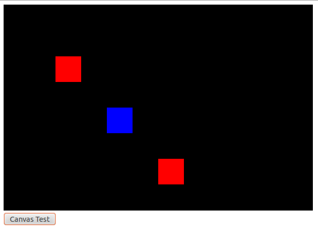
We can’t detect if two objects are touching each other without two objects to touch. And no object is easier to work with than a rectangle which can be represented as a single x and y coordinate (representing the upper-left corner of the rectangle) along with a width and height.

//Sample Rectangle Code: Don't Put In Your Game
var testRect = new Object();
testRect.x = 5;
testRect.y = 20;
testRect.width = 10;
testRect.height = 30;

Now if we build two objects like this we can test if they are touching or not with this neat little math function, which is logically equal to this function from Wikipedia.

//Test if two rectangles intersect
//Arguments are two objects which much have x, y, width and height variables
function intersectRect(r1, r2) {
   return !(r2.x > r1.x+r1.width ||
            r2.x+r2.width < r1.x ||
            r2.y > r1.y+r1.height ||
            r2.y+r2.height < r1.y);
}

This function runs four quick tests that can each prove that the two rectangles ARE NOT touching each other. The first line tests if the second rectangle is too far right to touch the first rectangle. The second line tests if the second rectangle is too far left to touch the first rectangle. The third line tests if the second rectangle is too low to be touching the first rectangle and finally the fouth line tests if the first rectangle is too high up to be touching the first rectangle.

If all the tests fail then the second rectangle must be touching the first rectangle and the function overall returns true. Come up with a few samples and run the logic by hand if you like. It’s not like this articles going anywhere.

How Many Hitboxes Does One Character Need?

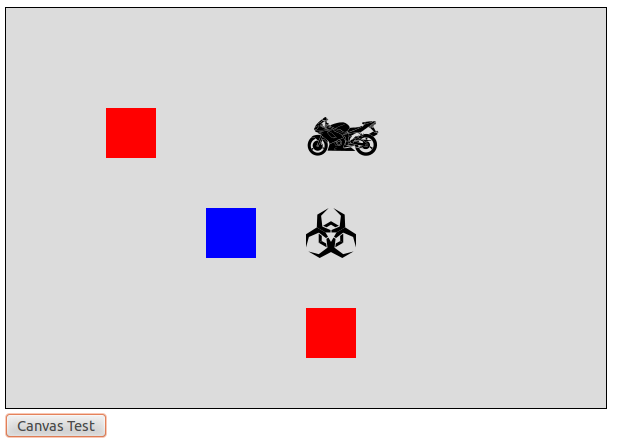
With that function we have everything we need to tell when rectangles collide. Now all we have to do is wrap all of our game graphics inside of invisible rectangles and it’ll be easy to tell when the player is running into enemies or crashing into platforms.

These invisible rectangles are called “hitboxes” and they are a vital game 2D* programming trick.

But there are certain problems with having your entire character represented by just one big hitbox.

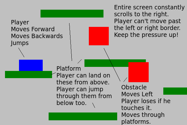
For example: Imagine You detect that your one-hitbox character has run into a one-hitbox floating block. What happens next should depend on what direction the character hit the block from.

If they collided with the block from above they should land on the block and treat it like ground.

If they collided with the block from below they should stop moving upwards and instead start falling down.

If they collided with the block from the side they should stop moving and then slide downwards.

But since the character has just one big hit-box it’s really hard to figure out what kind of collision just happened. All you know is that the character and the block are touching; you don’t know where they are touching or what part of the character hit the block first.

There is also the big issue that giving a character one big hitbox usually creates a hitbox that is larger than the character’s graphics. This can lead to frustrating scenarios where the player winds up dead because an attack hit the blank space near his character’s head. It looks like it shouldn’t count as a hit but it’s inside of the invisible hitbox so it counts.

One Hitbox Per Character: Simple But Flawed

So one big hitbox makes it hard to tell exactly what is going on with your character and can lead to frustrating collisions for the player. This is a problem!

The simple solution is to give each character multiple hitboxes for different logic.

Some common hitbox types include:

Death box: A small, central hitbox for checking whether attacks hit the player or not. By making it smaller than the character graphics we give the player a little wiggle room and avoid the “phantom hits” we would get if the hitbox covered whitespace.

Bonus Box: A large hitbox that is used for detecting whether the player has touched bonus items or not. Slightly larger than the player so that they can grab coins and power ups just by getting really close without having to worry about exact pixels.

Feet Box: A short but wide hitbox used for detecting whether the player is touching the ground. We put it in the bottom center of the sprite.

Head Box: A short but wide hit box used for detecting whether the player has just bumped his head against the ceiling. We put it at the top center of the sprite.

Side Boxes: Two tall but thing hit boxes used for detecting whether the player has run into a solid obstacle. We put them on the left and right sides of the player.

Multiple Hitboxes: Much More Elegant

Hitboxes For Defrag Cycle

So how many of those common hitbox types doe we need for our game? Let’s see…

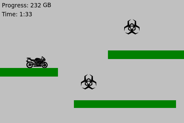
We need to be able to jump from platform to platform, so we’re going to need some sort of “foot hitbox” running along the bottom of the motorcycle.

We need to keep track of when the player runs into a virus and loses, so we’re going to need a small “death hitbox” in the center of the motorcycle.

We want to give players bonus points for grazing viruses, so we’re going to need a large “bonus hitbox” that’s actually a little bit bigger than the motorcyle. When a virus is inside this box but outside the “death hitbox” is when we give graze points.

We want players to be able to jump through platforms from below to land on top, so we DON’T need any sort of “head hitbox”.

The game has no walls, so we don’t need any “side hitboxes”.

So our final hitbox model for debug cycle has three hitboxes and will look something like this:

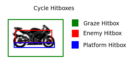
I think this should work

From Theory To Practice

Not a lot of code today, but that’s OK because we’ve laid down the groundwork we need to actually do some collision detection next time. Maybe throw is some gravity and get the player’s motorcycle to actually jump between platforms if I have the time.

* 3D games have a similar collision technique based around wrapping things with invisible cubes, cylinders and spheres.

Let’s Program A JavaScript Game 5: Press Start To Play

Posted on July 29, 2014 by Scott

Play A Game Or Watch A Movie?

Pop Quiz: What’s the main difference between a movie and a videogame?

If you answered “Player Input”: Congratulations, you’re exactly right! The main component that makes a game a game is the fact that the player has some control over what happens next. The player isn’t just watching some hero fight a monster, he’s pressing the buttons that make the hero fight.

If you answered anything else: You’re probably still right but that wasn’t the answer I was looking for so it doesn’t count. Try to do a better job of reading my mind next time I ask a semi-rhetorical question.

Anyways, my main point here is that player’s input is important and that’s what I’m going to be programming today.

Getting Input With JavaScript A.K.A. Whoops I Lied To You

Remember how we prototyped a getInput function and put it at the start of our gameLoop? Turns out that doesn’t work so great with JavaScript. Throw away that function and all references to it, we’re going to be doing something completely different.

Don’t look at me like that. This is a Let’s Program, I’m writing these articles at the same time as the code and I don’t always catch my mistakes early enough to fix them before hitting “post”.

Anyways, here is how it should work:

Instead of checking for input during the loop we will ask the browser to run a short piece of code every time a key is pressed. Of course, we may not be ready for player input at that exact moment so we will just have the code store the input for future use. That way if a player presses a key between game loops the input will still be there the next time we update.

As for the potential issue of the player pressing a key during a game loop… it’s not really a problem. Modern browsers can run multiple pieces of JavaScript at once so we don’t have to worry about the game lagging because it is trying to update the game and process input at the same time.

There is still the slight issue of what happens if player input changes halfway through a loop. Maybe the loop starts with the “right” key being pressed and then halfway through the key is released. This could lead to a strange state where we do 50% right key logic and 50% default logic. To prevent this we’ll just have to be sure that we only access player input once per loop so that it doesn’t have time to change on us, maybe by storing a local copy of player input at the start of every loop so that the global input can change without influencing the current frame.

Time For The Code

First off we have to let the browser know that we want the input. One easy way to do this is by adding onkeyup and onkeydown traits to the body tag in your HTML. Just change your code from this:

<body>

to this:

<body onkeydown="doKeyDown(event);" onkeyup="doKeyUp(event);">

Now everytime the user presses a key the browser will automatically run the doKeyDown function we’re about to write. And when they release a key it will automatically run the doKeyUp event that we are also about to code.

One warning: This will capture ALL keyboard input for that page, which is OK for a full page game but can be a bad idea if your game is just one part of a much larger page where people might want to use their keys for scrolling.

Capturing input doesn’t do us any good if we don’t have a place to store it, so let’s start by adding a new object declaration to the top of our script:

var playerInput = new Object()

Now we can write the doKeyDown and doKeyUp functions. They’re both pretty simple functions, with the only trick being that we have to double check whether the user is using Internet Explorer or not because certain code only works on certain browsers. Other than that we just check the numeric code of whatever button the user just pressed, see if the code matches any of the arrow keys and then record it in our playerInput variable.

function doKeyDown(event){
   var keynum;

   if(window.event){ //Browser is IE
      keynum = event.keyCode;
   }
   else{
      keynum = event.which;
   }

   if(keynum == 37){
      playerInput.left = 1;
   }
   else if(keynum == 38){
      playerInput.up = 1;
   }
   else if(keynum == 39){
      playerInput.right = 1;
   }
   else if(keynum == 40){
      playerInput.down = 1;
   }
}

function doKeyUp(event){
   var keynum;

   if(window.event){ //Browser is IE
      keynum = event.keyCode;
   }
   else{
      keynum = event.which;
   }

   if(keynum == 37){
      playerInput.left = 0;
   }
   else if(keynum == 38){
      playerInput.up = 0;
   }
   else if(keynum == 39){
      playerInput.right = 0;
   }
   else if(keynum == 40){
      playerInput.down = 0;
   }
}

Of course, if you are building a game that uses buttons other than the arrow keys you will need more else if statements for whatever buttons you are interested in. For example, maybe you want your running game to let the user use the spacebar to jump. To do so you’d just have to lookup the keycode for “space” and then keep track of a playerInput.space variable.

Introducing The Protagonist Square

We now have code for getting player input, but that’s no good without some way to test it. And while I suppose we could just print some logging text to the console that says “Player has pushed right arrow key” it would be much more fun to have some actual graphics moving around the screen.

So to start go up to the start of your script to where you declared the playerInput variable and add two new variables for xPos (x position) and yPos (y position). Let’s have them default to 100.

var xPos = 100;
var yPos = 100;

And now let’s use those variables to draw a red square on our screen by updating our screen drawing function like this:

//Draw the screen
function drawScreen(){
   var canvas = document.getElementById('gameCanvas');
   var context = canvas.getContext('2d');

   //Draw background
   context.fillStyle = '#dcdcdc';
   context.fillRect(0,0,600,400);

   //Draw black text
   context.fillStyle = '#000000';
   context.fillText("Loop Count: "+loopCount, 20, 20);

   //Draw a red square the player can control
   context.fillStyle = '#FF0000';
   context.fillRect(xPos, yPos, 50, 50);
}

And now we have a little red square that we can move around just by changing xPos and yPos. The logical next step is to use player input to change xPos and yPos, which we can do by rewriting updateGame like this:

function updateGame(){
   loopCount++;
   
   if(playerInput.right){
      xPos+=5;
   }

   if(playerInput.left){
      xPos-=5;
   }

   if(playerInput.up){
      yPos-=5;
   }

   if(playerInput.down){
      yPos+=5;
   }
}

Give It A Try

Save your changes, reload your game page and hit the “Canvas Test” button. You should see a red square appear on the screen, and the red square should move around when you press the arrow keys. If not you have some debugging to do. Make sure you copied the most recent functions correctly and that the playerInput, xPos and yPos variables are all properly declared inside the script tags but before you declare any functions.

And with that we’re done for this week. Next week I’ll probably talk about collision detection. Or maybe gravity. But since gravity isn’t really that useful without a ground to collide with I’m thinking it will probably be collision detection.

Let’s Program A JavaScript Game 4: V8 600HP Game Engine

Posted on July 22, 2014 by Scott

Reinventing The Wheel

Let’s be honest: Building our own game engine from scratch is probably not a great idea. There are already open-source JavaScript game engines that do everything we need but better. If you need to quickly and efficiently build a bug free JavaScript game looking at one of these existing solutions would definitely be your first step.

But this is a Let’s Program! Doing things from scratch and learning the hard way is our goal.

Your Game Comes With The Following Pieces…

When you get right down to it, all games are made up of the following two things:

Game Rules: How the game works.
Game State: What is going on in the game right now.

This is true for board games, card games and videogames.

In a board game the rules are usually written on the back of the box and the game’s state is where the pieces are on the board. In a card game the rules usually come in a little pamphlet and the state is the cards in each person’s hand. In a videogame the rules are built into the code and the state is kept track of by computer variables.

Conceptionally there is no real difference between Bob and Sally playing checkers by reading the back of a box and moving pieces around a board and Bob and his computer playing Grand Theft Auto by reading millions of lines of code and moving bits of data around inside memory.

Sure, a video game like Grand Theft Auto has dozens of “turns” per second to simulate real time action, but behind the scenes it’s still just the same old board-game mechanic of “follow the rules”, “make your move”, “update where the pieces are”.

How To Play The Game

Now that we’re all on board with the ideas of game rules and game state we can simplify running a game to a process of three repeating steps:

Check for player input
Update the game state based on the game rules and the player input
Redraw the screen based on the current game state

As an example, let’s imagine that the user presses the up key.

In step one the game checks for input and notices that the user has pressed the up key.

In step two it starts updating the game state. The game rules say that if the player presses the up key while standing on the ground he should “jump” by setting his up velocity to 20. The rules also say that the player and every enemy should move velocity pixels per update, so the game moves the player up 20 pixels and also moves two enemies on screen 10 pixels to the left. The rules also say the game should check for player/enemy collisions but the game doesn’t find any so it stops.

In step three the game now redraws the screen. It draws the player 20 pixels up in the air and draws the two enemies 10 pixels to the left of where they used to be.

50 milliseconds later the loop repeats.

In step one the game checks for input and notices that the user is still pressing the up key.

In step two the game checks the rules. The rules say that the up key only makes the player jump if he is standing on the ground, which he no longer is, so the input gets ignored. But the rules also say that characters in the air should have their velocity decreased by 5, so the player’s upward speed drops from 20 to 15. The game then updates all the characters, moving the player up by 15 pixels and the enemies left by 10. It checks for collisions and still doesn’t find any.

The game now redraws the screen. The player is now 35 pixels up in the air and the enemies are 20 pixels to the left of where they started.

50 milliseconds later the loop repeats a third time. And then a fourth time and a fifth time and so on.

Since the loop happens several dozen times a second the player gets the illusion that everything is happening in real time, but when you get right down to it the whole game could be converted into a turn-based boardgame no problem. Not that anyone would want to play a boardgame where it takes a few hundred turns to cross a room and the rulebook is written mostly in math terms… but the idea is still sound.

Looping In Javascript

Warning: We’re going to be experimenting with loops. Odds are good that you will make a mistake, create a crazy infinite loop, freeze your browser and have to force it to shut down. So don’t panic if your test page suddenly stops responding. Just close the browser and double check whatever code you just typed in.

Now our final goal for the game loop is to have it run once every 50 milliseconds. That’s 20 times a second, which is honestly a little on the low side for a video game but still high enough to feel like smooth-ish animation and interaction. Most importantly it’s slow enough that we can basically guarantee our code will complete inside of each loop, giving us plenty of wiggle room when prototyping messy code. After that’s done we can always go back and adjust the loop to run more often if the game feels too jerky.

Now the most obvious approach to make a loop run once every 50 milliseconds would be be to use “setInterval”, which allows us to schedule a function to repeat again and again every X milliseconds. It sounds perfect and this approach can work. I’ve used it in demo games before.

But running the algorithm once every 50 milliseconds does have one big issue: What happens if your function takes longer than 50 milliseconds? You can wind up in a situation where setInterval triggers a new game loop while the old one is still running, which is a bad bad thing. Having two functions trying to control your game at the same time can corrupt variables, double move characters and generally mess everything up.

To avoid this we will use this strategy instead:

Check what time it is at the start of our game loop.
Check what time it is at the end of our game loop.
If more than 50 milliseconds have passed, immediately call the game loop function again.
If less than 50 milliseconds have passed, use setTimeout, which lets us schedule a function to be called only once after a timer runs out.

Because we don’t schedule the next game loop until after we know the current game loop has finished we can now guarantee that we will never end up with multiple game loops interfering with each other. If a loop takes longer than 50 milliseconds we just wait for it finish before moving on. This will cause slight lag, but that’s better than having the engine actually break.

Now on to the nitty gritty technical details. When using setTimeout the first argument has to be a STRING copy of the code you want to run and the second argument is how many milliseconds the browser should wait before running it.

Making sure the first argument is a string is important. If the first argument is actual code it will be called immediately* instead of after the timer goes off. You can see this for yourself by experimenting with code like this:

//Wrong! The alert is called immediately
setTimeout(alert('Time Is Up!'), 2000);
//Right! The code inside the string gets called after two seconds
setTimeout("alert('Time Is Up!')", 2000);

The big risk here is creating infinite loops. For instance, our upcoming gameLoop function ends by scheduling another gameLoop. If you accidentally call gameLoop immediately instead of properly quoting it and scheduling it for later you will end up with an infinite loop of hyper-fast gameLoops instead of the steady one-loop-per-50-milliseconds you were hoping for. This will also probably freeze your browser. Happened to me. Don’t let it happen to you.

Prototyping The Loop

Open up the test code from two posts ago and replace whatever script you had with this:

var loopCount=0;

function canvasTest(){
   gameLoop();
}

//The main game loop
function gameLoop(){
   var startTime = Date.now();
   getInput();
   updateGame();
   drawScreen();

   var elapsedTime = Date.now()-startTime;
   if(elapsedTime>=50){ //Code took too long, run again immediately
      gameLoop();
   }
   else{ //Code didn't take long enough. Wait before running it again
      setTimeout("gameLoop()",50-elapsedTime);
   }
}

//Get the player's input
function getInput(){
   //Empty prototype
}

//Update the game by one step
function updateGame(){
   loopCount++;
}

//Draw the screen
function drawScreen(){
   var canvas = document.getElementById('gameCanvas');

   var context = canvas.getContext('2d');
   
   //Draw background
   context.fillStyle = '#dcdcdc';
   context.fillRect(0,0,600,400);

   //Draw black text
   context.fillStyle = '#000000';
   context.fillText("Loop Count: "+loopCount, 20, 20);
}

Now click the “Canvas Test” button and watch that counter climb at a speed of approximately 20 loops per second.

Let’s walk through the code really fast.

Clicking the button triggers canvasTest like usual, and canvasTest calls gameLoop.

gameLoop takes a note of what time it is (in milliseconds) by calling Date.now. The game loop then runs the three steps of our game (get player input, update game, and draw screen) and then checks how much time has passed by comparing the stored “startTime” to a second call to Date.now. If 50 or more milliseconds have passed we are running slow and need to call gameLoop again immediately. Otherwise we set a timer and have gameLoop run again later.

The three steps of the game are pretty empty at this point. We don’t care about player input so we leave that function blank. Our only game update is to increase the global “counterLoop” and painting the screen involves nothing but redrawing the background and printing a message about how many loops we have seen.

Next Time: Let’s Get Interactive

We’ve just built a simple but serviceable game engine skeleton. Now it’s time to start filling in the prototype functions, starting with getInput. Join me next week to see how that goes.

* There is one scenario where putting a function call in setTimeout would be a good idea: When the function’s main purpose is to return a string containing the code you actually want to schedule. Maybe you have a “builScheduledCode” function that returns different string wrapped functions depending on the state of the program. Like, if the debug flag is set it returns “logState();runLogic();” but if the debug flag is clear is only returns “runLogic()”;

Let’s Program A JavaScript Game 3: Designing “Defrag Cycle”

Posted on July 15, 2014 by Scott

Some Obvious Game Design Theory

Videogames are a combination of gameplay and theme.

In Dragon Quest, an RPG, gameplay consists of exploring grids, navigating menus and trying to make your team’s numbers go up while the enemy team’s numbers go down. But the theme is “Fantasy Adventure” which turns the grids into dungeons and the number manipulations into tense combat with all sorts of magic and monsters.

In Counter Strike, an FPS, gameplay is all about moving around a big piece of geometry and trying to tag other players with various vectors. But the theme turns the geometry into a modern day battlefield and the vector tagging into guns and bullets.

When designing a game sometimes you start with a gameplay idea and then come up with a theme that fits it. Other times you start with a theme in mind and then come up with gameplay that lets you tell the story you want. And quite often the theme and gameplay evolve together in the designer’s mind, each one influencing the other.

Designing Our Gameplay

For this Let’s Program we’re going to take a “Gameplay First” approach to design. Mostly because we’re here as programmers and as programmers our main focus is on writing interesting code, not writing interesting stories. We can talk about the fine art of game theme design some other time.

One easy way to design a game is to play a lot of other games and then adopt (a.k.a. shamelessly copy) whatever gameplay elements you enjoy the most. This Let’s Program is going to focus on the “Running” genre of casual browser games. These are games where the player controls an avatar that constantly runs to the right and the player’s goal is to jump over various obstacles in order to see how far they can go.

Here are a few examples (built using Flash, not JavaScript, but you get the idea):

These games were both built by people with significantly more time and artistic talent than me, so my final product isn’t going to look anywhere near as nice or have as many special features. But I will still be following the same basic gameplay pattern.

A Picture Is Worth A Thousand Words

OK, so the basic idea is that the player has to move along a path while avoiding obstacles. In my game the two main obstacles are going to be:

Gaps in the path
Moving projectiles

In order to avoid these obstacles the player can move left, right and perform simple jumps. To help keep the pressure on the player the entire screen will scroll constantly, forcing them to keep moving. We will also make the game get harder as it goes on by making the projectiles faster and the platforms smaller as time goes on.

Here are a couple rough pictures that help explain the gameplay I’m aiming for.

Try to imagine all the pieces moving around

Try making some sound effect noises while looking at this picture. It helps.

Introducing: Defrag Cycle!

Now that we have the basic gameplay under control we can start working on adding a theme to the game.

Our gameplay is pretty basic and with the right art you could turn the game into just about anything. A hero jumping along cliffs while avoiding fireballs. A ninja jumping from tree to tree while avoiding shurikens. Or even something completely crazy like a plumber jumping around on pipes while avoiding flying turtles.

But I can’t draw, so my choice of game themes is somewhat limited. I’m going to have to rely on free clipart for all my graphics, like the motorcycle and virus from the canvas tutorial.

In fact, let’s use those two exact graphics. What kind of game theme can we come up with that involves a motorcycle and a bunch of viruses?

How about… the motorcycle represents a “defragmentation” computer program that helps clean up hard drives. The obstacle course that the player has to navigate represents a fragmented hard drive and the viruses represent (obviously) computer viruses. The player’s goal is to completely defrag the harddrive by avoiding the viruses and not failing off the path.

Yeah, I realize it sounds kind of like Tron. But is that really a bad thing?

Anyways, the game will have two score counters: a “progress” and a “time”. Both will automatically go up as long as the player isn’t dead. When the “progress” count reaches 1,000 GB the hard drive is completely defragged, the player wins and their total time is shown.

To help reward good players we will introduce a “graze” mechanic where people who get really close to a virus without actually colliding with it will be awarded bonus “progress” points. This will let good players defrag the hard drive faster than usual and give them a much lower total time.

Here are a couple screen shots of what I had in mind:

Not bad for a game built entirely around two pieces of free clipart

I don’t actually like games with graze mechanics. Why am I doing this? What I have become!?

Next Time: Start Your (Game) Engines

Now that we have a basic game design document we can start to actually program our game. So join me next week as we take the first step towards building the custom JavaScript we need to actually run our game.

Let’s Program A JavaScript Game 2: The Canvas Of Dreams

Posted on July 8, 2014 by Scott

Let’s Program A JavaScript Game 2: The Canvas Of Dreams

No Time For HTML

This is “Let’s Program A JavaScript Game” not “Let’s Program A Website” so instead of discussing the fine points of HTML structuring I’m just going to drop the code for a very basic skeleton page that we can use for testing out the canvas. Just type or copy the following text into a file named something like “javascriptgame.html” and then open it up with your favorite modern browser (most up to date browsers support the canvas):

<!DOCTYPE html>
<html>
<head>
   <script>
      function canvasTest(){
         alert("Canvas Test");
      }
   </script>
</head>
<body>
   <canvas id="gameCanvas" width=600 height=400></canvas>
   <br/>
   <button onclick="canvasTest()">Canvas Test</button>
</body>
</html>

Not much to this. The HTML document has a HEAD, that holds our script, and a BODY that holds our canvas and one button. Clicking the button calls our script and if everything works properly you should get a screen sort of like this:

Just a quick test to make sure your button is connected to the script

Paint It Black

The first step to actually doing something interesting with our canvas is to put a reference to the canvas inside of a JavaScript variable. Then we use that reference variable to create a “context” object that can be used to do the actual work.

With our context all set up painting the entire canvas is as simple as setting the fillStyle of our context to whatever color we want and then calling the fillRect function. This function needs four arguments: the x and y coordinates of the top-left corner of the rectangle you want to draw along with the width and height of the rectangle.

Here’s our updated canvastTest function and a picture of what it should do. Remember to refresh the page in order to get the new code into the browser. If clicking on the button just shows the alert again odds are the old page is still in your browser memory and refreshing is the easiest way to force it to get rid of the old and grab the new.

function canvasTest(){
   var canvas = document.getElementById('gameCanvas');
   var context = canvas.getContext('2d');
   context.fillStyle = '#000000';
   context.fillRect(0,0,600,400);
}

A boring but important first step: Painting the entire canvas all one color

Paint It Black, But With Polka Dots

Painting the entire screen black is kind of boring. Let’s add some color now by choosing a new fillStyle and then drawing some more rectangles on top of the black background rectangle.

Here’s an updated canvasTest that draws two red squares and a blue square when we hit the button:

function canvasTest(){
   var canvas = document.getElementById('gameCanvas');
   var context = canvas.getContext('2d');

   //Draw background
   context.fillStyle = '#000000';
   context.fillRect(0,0,600,400);
 
   //Draw red object
   context.fillStyle = '#ff0000';
   context.fillRect(100,100,50,50);
   context.fillRect(300,300,50,50);

   //Draw blue object
   context.fillStyle = '#0000ff';
   context.fillRect(200,200,50,50);
}

Notice that when drawing the two red squares we only had to set the fillStyle once.

Colorful Geometry Is Colorful

Graphics And Sprites And Images, Oh My!

Drawing colored boxes is nice, but not quite enough for a full game. People expect their games to actually look like things; the box has to be a robot or a soldier or an alien or an alien-robot-soldier.

So let’s add some graphics to this demo using these two bits of clipart I found on a free clipart website*. You’ll need to save them to the same folder as your code if you want to keep following along.

Before we can draw these images to the canvas we need to load them into our code, which we do easily enough by adding a few lines to the top of our script that will be automatically run when the page loads. But watch out! Loading images over the Internet can take a long time and trying to draw an image before loading it will crash your game. This won’t be a problem for your test, since the graphics are small and already on your computer, but for an actual online game with lots of graphics it can be a real problem. We’ll talk about how to fix that later.

Once the images are loaded drawing them to the screen is as easy as a call to drawImage. Note that I also changed the color of the background so that the black clipart shows up better. Otherwise you’ll have two black images on a black screen and you’ll have no way to tell if it’s working or not.

var cycleImage = new Image();
cycleImage.src = "cycle.png";

var virusImage = new Image();
virusImage.src = "virus.png";

function canvasTest(){
   var canvas = document.getElementById('gameCanvas');
   var context = canvas.getContext('2d');

   //Draw background
   context.fillStyle = '#dcdcdc';
   context.fillRect(0,0,600,400);

   //Draw red object
   context.fillStyle = '#ff0000';
   context.fillRect(100,100,50,50);
   context.fillRect(300,300,50,50);

   //Draw blue object
   context.fillStyle = '#0000ff';
   context.fillRect(200,200,50,50);

   //Draw Images
   context.drawImage(cycleImage, 300, 100);
   context.drawImage(virusImage, 300, 200);
}

Motorcycles are cool! Hazard symbols are cool!

Animation! Sort of!

We’ve actually more or less covered everything we need to know to start prototyping our game. But just for fun let’s update our function to be “animated”: Every time you click the button the squares and clipart will move. We do this by creating a global “offset” variable right before our function. By adding an offset to the x or y coordinates of our drawings we can move them around the screen, and by constantly increasing the offset we can create the illusion that they are steadily moving in one direction.

So change your script to this and then click the “Canvas Test” button a few dozen times and see what happens.

var offset=0;

var cycleImage = new Image();
cycleImage.src = "cycle.png";

var virusImage = new Image();
virusImage.src = "virus.png";

function canvasTest(){
   var canvas = document.getElementById('gameCanvas');
   var context = canvas.getContext('2d');

   //Draw background
   context.fillStyle = '#dcdcdc';
   context.fillRect(0,0,600,400);

   //Draw red object
   context.fillStyle = '#ff0000';
   context.fillRect(100+offset,100,50,50);
   context.fillRect(300+offset,300-offset,50,50);

   //Draw blue object
   context.fillStyle = '#0000ff';
   context.fillRect(200,200-offset,50,50);

   //Draw Images
   context.drawImage(cycleImage, 300 - offset, 100);
   context.drawImage(virusImage, 300 + offset, 200);

   offset+=10;
}

A few things worth noticing here:

When two objects overlap whichever one comes last in the code gets drawn last and shows up on top. Example: The blue and red square
When an object is partially outside the canvas the part inside the canvas still gets drawn
You can “draw” an object completely outside of the canvas without breaking anything. It just doesn’t show up.

Time To Decide What To Do With All This Cool Code

So we can draw screens now and have even covered the basics of animation. We’re basically all set to start building our game!

Or we would be if we had any idea what we were going to build. So next week I’m going to take some time and lay out a simple game design document.

* Original images can be found here:

https://openclipart.org/detail/191534/motorcycle-silhouette-vector-by-raimondi1337-191534

https://openclipart.org/detail/28408/malware-hazard-symbol-by-pbcrichton

Let’s Program A Swarm Intelligence: Index And Code

Posted on June 24, 2014 by Scott

Introduction

Welcome fellow AI enthusiasts. Have you ever heard the phrase “Swarm Intelligence” and wondered just exactly what that means? Then wonder no more because I have here for you a whole set of articles about how to use swarm intelligence techniques to build a flexible AI capable of optimizing a wide variety of mathematical problems and real world equations.

Basically it all boils down to something like this:

An animation of a swarm optimizing a sine wave based function

A really cool looking swarm intelligence

Index

Let’s Program A Swarm Intelligence 1: Introducing Particle Swarm Optimization

Let’s Program A Swarm Intelligence 2: Learning To Love Lisp

Let’s Program A Swarm Intelligence 3: All Your Max Are Min

Let’s Program A Swarm Intelligence 4: Specifying A Use Case

Let’s Program A Swarm Intelligence 5: Defining The Swarm

Let’s Program A Swarm Intelligence 6: Assembling The Swarm

Let’s Program A Swarm Intelligence 7: Satisfying My OCD

Let’s Program A Swarm Intelligence 8: It Lives!

Let’s Program A Swarm Intelligence 9: All Together Now

Let’s Program A Swarm Intelligence 10: Let Me See…

Let’s Program A Swarm Intelligence 11: Turning Your World Upside Down

Let’s Program A Swarm Intelligence 12: Is That A Trick Question?

Let’s Program A Swarm Intelligence 13: Welcome To The Nth Dimension

Let’s Program A Swarm Intelligence 14: Better Particles, Better Swarm

Let’s Program A Swarm Intelligence 15: The Return Of Maximize And Target

Let’s Program A Swarm Intelligence 16: The Swarm Ate My Homework

Complete Code

If you follow along with the posts you should be able to write your own swarm intelligence from scratch in whatever programming language you want. But if you don’t have the time for that or just want some reference code I have also provided my completed code: Lisp Swarm Intelligence

Let’s Program A Swarm Intelligence 16: The Swarm Ate My Homework

Posted on June 24, 2014 by Scott

The Freshman Math Challenge

After roaming around on the Internet for a while I found a website offering open source college material including a rather decent worksheet on multi-variable optimization, which you can find here http://ocw.capilanou.ca/mathematics-statistics/math-109-calculus-ii/optimization-problems.pdf/view?searchterm=optimization.

I’ll be using problems from this worksheet to test out the swarm. Let’s see if we’ve built a machine smart enough to pass an entry level calculus class.

Profit Optimization

First problem from the worksheet is pretty straightforward. There is a random desk company that sells both finished and unfinished desks, although I’m not actually sure what they mean by this. Are they talking about whether or not the wood on the desk is properly stained, or by unfinished do they mean that they literally sell desks that are still missing pieces? Is there a big market for three legged desks?

Anyways, whatever an “unfinished” desk is the company’s revenue looks like this:

revenue = 200*finished + 160*unfinished – 0.2*finished*unfinished – 0.2*finished^2 – 0.25*unfinished^2.

The company’s expenses look like this

expense = 100*finished + 70*unfinished + 4000

The company’s profit is equal to its revenue minus its expenses, which we can represent as this Lisp function:

;Revenue for a company which sells both finished and unfinished furniture
(defun company-profit (fin unfin)
   (let ((revenue (+ (* 200 fin) 
                     (* 160 unfin) 
                     (* -0.2 fin unfin) 
                     (* -0.2 fin fin) 
                     (* -0.25 unfin unfin)))
         (expense (+ (* 100 fin) (* 70 unfin) 4000)))
      (- revenue expense)))

Now we just have to decide on some boundaries for our swarm guesses. Since you can’t produce less than 0 units of furniture our minimum bound for both types of desks will be 0. When it comes to the upper bounds we’ll have to take a bit of a guess. The bigger the boundary the larger our swarm will need to be to explore it and the longer the search will take, so we want to aim for an upper boundary that is small enough to be efficient while still being large enough to capture the maximum number of desks a company can reasonably build in one week.

Let’s start out with an upper bound of 10,000. That’s a pretty large number of desks for a small company to produce in a single week, so we should be safe. On the other hand, if that number is too small we’ll probably get an optimal solution right on the edge of our boundaries. If that happens we’ll just increase the boundaries and try again.

Now it’s time to put that all into action:

[5]> (defparameter *swarm-iterations* 200)

*SWARM-ITERATIONS*

[6]> (defparameter *swarm-size* 1000)

*SWARM-SIZE*

[7]> (defparameter *swarm-output* (swarm-maximize #’company-profit ‘((0 10000) (0 10000))))

*SWARM-OUTPUT*

[8]> (first *swarm-output*)

(200.04425 100.01073)

So it looks like the swarm thinks we should build 200 finished desks and 100 unfinished desks. And if we scroll down to the answer key portion of the worksheet that turns out to the right answer. Good job swarm!

Minimize Distances

Now let’s jump down to problem 3. A power station is being planned and they want to figure out the best place to put it so it can efficiently serve three different communities. Apparently this means they want to minimize the sum of the squares of the distances to each of the three communities which are positioned at (-4, 4) (5, 2) and (-1, -3).

Writing a function to calculate the sum of squares isn’t too hard, especially if we use the expt function to square things and the sqrt function to take square roots. Just remember that distance can be calculated by taking the square root of the square of the X and Y distances between two points and the following function should make perfect sense.

;Calculate the sum of squares of distances between a given point and the three points (-4, 4) (5, 2) and (-1, -3)
(defun sum-of-squared-distances (x y)
   (let ( (distance1 (sqrt (+ (expt (- x -4) 2) (expt (- y 4) 2))))
          (distance2 (sqrt (+ (expt (- x 5) 2) (expt (- y 2) 2))))
          (distance3 (sqrt (+ (expt (- x -1) 2) (expt (- y -3) 2)))))
      (+ (expt distance1 2) (expt distance2 2) (expt distance3 2))))

Time to choose our boundaries. Since we want to minimize the distance between the plant and the communities the power plant should logically be somewhere in the middle of the three points. So by looking at our points this means our x boundary needs to be between -4 and 5 and our y boundary needs to be between -3 and 4.

Time to let the swarm loose.

[29]> (defparameter *swarm-size* 25)

*SWARM-SIZE*

[30]> (defparameter *swarm-iterations* 100)

*SWARM-ITERATIONS*

[31]> (defparameter *swarm-output* (swarm-minimize #’sum-of-squared-distances ‘((-4 5) (-3 4))))

*SWARM-OUTPUT*

[32]> (first *swarm-output*)

(-7.074524E-4 1.0000945)

According to the swarm the best place for the power plant is around (0, 1), which matches up with the answer key. Another victory for the swarm!

A Problem With Extra Requirements

Now let’s go back to problem 2. This one turned out to be rather tricky.

At first it looks like a pretty simple. We have a package with length, width and depth (like all 3D objects). We want to maximize the volume. Just a simple 3 variable maximization, right?

Except that postal regulations require that the length and girth of the box have to add up to less than 108 inches. Or as the worksheet is happy to summarize: 2x + 2y + z <= 108.

This is a problem because our swarm is designed to make completely random guesses for x, y and z. We can give it some general guidelines like “x has to be between 0 and 10” but we can’t give it a complex constraint like “x plus y plus z needs to be less than 100”.

So at first it seems like our swarm just isn’t smart enough for this problem. But maybe there is a clever way around this issue. Take a look a this function:

;Calculates the volume of a package that has to have a combined length and girth of less than 108
(defun postal-package-volume (x y z)
   (if (> (+ (* 2 x) (* 2 y) z) 108)
       -1
       (* x y z)))

If the user tries to calculate the volume of a package that’s too big to mail we return -1 instead of the volume. Not only is this a good way to let a human know that there is a problem with their input, it also works great with our swarm. Since we want to maximize volume an “error” value of -1 will always be considered less optimal than even the worst of “acceptable” answers, all of which are positive.

In other words, instead of trying to prevent the swarm from making unacceptable guesses we just make sure that unacceptable guesses are always less optimal than acceptable guesses.

Time to see if it works. Our boundaries are based off the fact that a box can’t have negative length and that the definition of girth means that 54 is the biggest x and y values possible and that 108 is the biggest possible z.

[44]> (defparameter *swarm-size* 25)

*SWARM-SIZE*

[45]> (defparameter *swarm-iterations* 100)

*SWARM-ITERATIONS*

[46]> (defparameter *swarm-output* (swarm-maximize #’postal-package-volume ‘((0 54) (0 54) (0 108))))

*SWARM-OUTPUT*

[47]> (first *swarm-output*)

(17.743437 18.024296 36.464497)

If we look at the answer key the true maximum is (18, 18, 36), which is pretty close to the swarm’s guess. Looks like our workaround for the input constraints worked!

Conclusion And Extra Challenges

That’s it. We wrote a general swarm optimizer smart enough to ace a freshman calculus assignment. So while our swarm isn’t anywhere near being a professional quality artificial intelligence I think it’s more than good enough to be considered a successful “Let’s Program”.

Of course, I’m sure there are plenty of you out in the audience who don’t want to stop here. If you want to forge on ahead on your own here are a few sample projects you might want to consider tackling next:

Find more complicated optimization problems that require more than 3 variables. Does the swarm find the right answer? If not, fix it until it does.
Improve particle behavior by giving them memory of their personal best answer and having them adjust their velocity based on a combination of current velocity, swarm best and personal best.
Create multiple types of particles, such as scout particles that don’t care so much about the swarm best and random particles that bounce around problem space even when the rest of the swarm has settled on a possible best answer. This would be a great place to practice object oriented programming.

And with these final suggestions I bid you adieu. All that’s left is the index page. Thanks for following along!

Let’s Program A Swarm Intelligence 15: The Return of Maximize and Target

Posted on June 16, 2014 by Scott

Solving A Problem We Already Solved

Last post we upgraded our swarm so that it could successfully minimize problems with any number of variables. All that’s left now is to teach it how to maximize and how to aim for specific results.

By now you should understand that maximization is just minimization turned upside down and hitting a target is the same as minimizing the difference between the results you are getting and the results you want.

Thanks to this insight we were able to easily write a 2D maximizer and target seeker by just using our already written minimizer. Now it’s time to do the same thing for the general swarm.

The tricky part here has to do with arguments.

In the 2D swarm we knew that everything would have two variables, so we were able to use lambda to build new two variable functions on demand. Then we passed that new two variable function to swarm-minimize-2d, which gave it the two arguments it expected.

But this time things are different. The general swarm-minimize uses apply to pass an unpredictable number of variables to our function. Which means that the new lambda function we build has to be able to accept a flexible number of variables and then pass them all on the the original function.

Fortunately for us Lisp is all ready to handle this problem thanks to the keyword &rest. Put inside of a function declaration this basically means “A list of every extra variable in the function call”.

A quick demo:

(defun rest-test (first second &rest extra)
   (format t “This is the first argument: ~a~%” first)
   (format t “This is the second argument: ~a~%” second)
   (format t “There were ~a extra arguments:~%” (length extra))
   (loop for argument in extra do (format t “~a~%” argument)))

[9]> (rest-test “one” “two” “three”)

This is the first argument: one

This is the second argument: two

There were 1 extra arguments:

three

NIL

[10]> (rest-test “one” “two” “three” “four” “five”)

This is the first argument: one

This is the second argument: two

There were 3 extra arguments:

three

four

five

NIL

This is exactly what we need in order to create a lambda function that can take a flexible number of variables and pass them all along to an inner function. Upgrading the 2D maximize and target functions is now simple:

(defun swarm-maximize (fn boundaries)
   (swarm-minimize (lambda (&rest arguments) (* -1 (apply fn arguments) boundaries))))

(defun swarm-target (fn target boundaries)
   (swarm-minimize-2d (lambda (&rest arguments) (abs (- target (apply fn arguments)))) boundaries))

Let’s take these new functions for a spin:

[16]> (defparameter *swarm-iterations* 100)

*SWARM-ITERATIONS*

[17]> (defparameter *swarm-output* (swarm-maximize #’inverse-double-parabola ‘((-10 10)(-10 10))))

*SWARM-OUTPUT*

[18]> (first *swarm-output*)

(5.114901E-5 4.665053E-7)

[19]> (defparameter *swarm-output* (swarm-target #’triple-parabola 7 ‘((-10 10)(-10 10)(-10 10))))

*SWARM-OUTPUT*

[20]> (first *swarm-output*)

(-1.5512012 0.78995675 -1.9924128)

[21]> (triple-parabola -1.5512012 0.78995675 -1.9924128)

6.9999657

Success on both counts!

Coincidentally, this also shows off that our general swarm optimizer can handle 2D problems just as well as the specific 2D swarm optimizer. This is nice because it let me test maximization on a function we already had and saved me the trouble of writing an inverse triple parabola.

Time To Give The Swarm A Real Run For It’s Money

Ok, so we were able to maximize and target a couple of parabolas using the general swarm. But that’s not really very impressive. Parabolas are easy to solve and these weren’t even high dimensional problems.

So for my next and final “Let’s Program A Swarm Intelligence” I’m going to pull out all the stops and try to find some real world multi-variable problems to test this thing on. I’m sure I have a few engineering and calculus textbooks laying around with interesting problems just waiting to be solved.

Let’s Program A Swarm Intelligence 14: Better Particles, Better Swarm

Posted on June 10, 2014 by Scott

The End Is Near

Last time we successfully upgraded our particle objects to be flexible enough to work in any number of dimensions so they can help us optimize problems with any number of variables. Now all we need to do is upgrade our old 2D swarm algorithms to use these new super-particles and we’ll have a complete, generalized particle swarm optimizer.

Fair warning: A lot of the code in this post looks really complicated. And I guess it kind of is. But remember that everything we are doing in this post is something we’ve already done successfully in two dimensions and that the basic logic is the same. Just remember the basics of swarm logic (make a lot of guesses, update your guesses, repeat) and you should be fine.

Also, we can’t really develop a general swarm optimizer without a few multi-variable problems to test it on. So behold, Multi-dimensional parabolas!

(defun triple-parabola (x y z)
   (+ (* x x) (* y y) (* z z)))

(defun quadruple-parabola (x y z w)
   (+ (* x x) (* y y) (* z z) (* w w))

Once again the obvious minimum for both these problems is when all the inputs are set to 0. That’s (0, 0, 0) for the triple parabola and (0, 0, 0, 0) for the quadruple parabola. Hopefully the swarm will be able to figure that out too.

A More General Swarm Definition

The first step in upgrading our particles was to remove specific references to 2D ideas like X and Y and then replace them with flexible lists that can grow to whatever size the problem demands. Similarly the first step in upgrading the swarm itself is to remove specific 2D references and replace them with more flexible structures.

The big change here is that our 2D swarm used to keep track of the best X and Y coordinates any particle had found so far. We will now replace those with one “best-coordinates” variable that we will use to store a copy of the entire coordinates list of any particle that manages to find a good possible answer. This way we can have one variable that works no matter how long the coordinate list gets.

(defclass swarm ()
   ((best-coordinates
       :accessor best-coordinates
       :initform nil)
    (best-answer
       :initarg :best-answer
       :accessor best-answer
       :initform most-positive-long-float)
    (particle-list
       :accessor particle-list)))

Next up is creating a handy swarm generating function. Just like with the particle generator function the main focus of this upgrade will be to remove specific references to X and Y limits and replace them with a flexible “boundaries” list that will include a min and max pair for every variable in the problem we are minimizing.

(defun generate-swarm (particle-count boundaries)
   (let ((new-swarm (make-instance 'swarm)))
      (setf (particle-list new-swarm)
            (loop for i from 1 to particle-count
             collect (generate-particle boundaries)))
      new-swarm))

Most of the hard “boundaries” work was already done inside of generate-particle so this upgrade was as easy as swapping out a few old variables for a new one and making sure that “new-swarm” is created as a swarm object instead of a swarm-2d object.

Same Logic, More Numbers

Upgrading the swam logic is pretty easy. We just replace the idea of x-limit and y-limits with a single boundary variable and then switch to the non-2D version of every function call.

(defun swarm-minimize (fn boundaries)
   "A general particle swarm optimizer"
   (let ((swarm (generate-swarm *swarm-size* boundaries)))
      (loop for i from 1 to *swarm-iterations* do
         (loop for particle in (particle-list swarm)
           do (update-swarm-particle particle swarm fn boundaries)))
      (list (best-coordinates swarm) (get-swarm-history swarm))))

Only problem is… not all of these functions exist yet. So before swarm-minimize can actually be used for anything we’re going to have to write our new generic update-swarm-particle. Watch out because this one is a doozy!

(defun update-swarm-particle (particle swarm fn boundaries)
   (update-particle-history particle)
   (let ((particle-answer (apply fn (coordinates particle))))
      (when (< particle-answer (best-answer swarm))
         (setf (best-answer swarm) particle-answer)
         (setf (best-coordinates swarm) (coordinates particle))))
   (update-particle-velocity particle (best-coordinates swarm))
   (setf
      (coordinates particle)
      (loop
         for position in (coordinates particle)
         for velocity in (velocity particle)
         for bounds in boundaries
         collect (max (first bounds) (min (second bounds) (+ position velocity))))))

Let’s start with the easy changes. We switch from update-particle-history-2d and update-particle-velocity-2d to the more general versions that we’re about to write. We also switch from funcall to apply for generating the answer associated with a particular particle position. apply is basically a funcall that expects it’s input in a list instead of typed out as individually which works really great now that our input is all in a list.

Then comes the hard part: updating particle positions. We used to just manually update X and Y position based of of X and Y velocity and X and Y limits, but we need more flexibility than that now that our coordinates, velocity and limits are all stored in lists instead of predictable variables.

Once again we’re going to turn to the mighty loop macro to solve this list based problem. Our goal is to process an entire list of coordinates using an entire list of velocities and in order to do that we’re going to take advantage of a handy loop trick that lets us iterate over multiple collections at the same time. You just include more than one “for variable in collection” inside the start of your loop and then every time you go through the loop you get one item from every collection. The first time through the loop you get the first item from every collection, the second time you get the second item from every collection and so on.

This is great because in order to update a particle we need to be able to update the first coordinate by using the first part of velocity and then making sure the result is inside of the first boundaries. Then we need to update the second coordinate with the second part of velocity and the second set of boundaries. So on with the third and fourth and however many dimensions we have. It’s the perfect place for the multiple-collection-loop trick.

Anyways, the end result of all our looping is to calculate a set of new coordinates, collect them into a big list and then replace the old particle coordinate list with the updated one.

Of course, the above function won’t work without an update update-particle-velocity, so let’s tackle that next. Its upgrade requires the same sort of loop tricks so if you understood the last function this one will be even easier. If you didn’t understand the last function, carefully read through it again.

(defparameter *original-velocity-weight* 0.8)
(defparameter *target-velocity-weight* 0.3)

(defun update-particle-velocity (particle target-coordinates)
   (setf
      (velocity particle)
      (loop
         for original-velocity in (velocity particle)
         for position in (coordinates particle)
         for target in target-coordinates
         collect (let ((target-velocity (- target position)))
                    (+ (* *target-velocity-weight* target-velocity)
                       (* *original-velocity-weight* original-velocity))))))

Let’s remember back to how the 2D version of this function worked. For both X and Y we compared where the particle currently was to where the swarm’s best answer so far was and used this to calculate a target-velocity that would lead the particle to the best answer. We then took some fraction of this target seeking velocity and added it to some fraction of the particle’s original velocity. This meant that over time particles would eventually gravitate towards the swarm best.

The generic version uses a loop to do the same thing. It grabs one component of its current velocity, one component of its current position and one component of the target swarm-best coordinate. It then calculates a target-velocity for just that one portion of the velocity, mixes it in with the current velocity and collects the whole thing into the new velocity list that we eventually set as the particles new velocity. In other words, if we were solving a 3D three variable problem the first trip through the loop would use X position, X velocity and X best-coordinates to calculate a new X velocity. Then the second loop would update the Y velocity and the third loop would update the Z velocity.

With that tricky function out of the way all that’s left are a couple useful history related helper functions:

(defun update-particle-history (particle)
   (setf
      (history particle)
      (append
         (history particle)
         (list (coordinates particle)))))

(defun get-swarm-history (swarm)
   (loop for particle in (particle-list swarm)
    collect (history particle)))

The first is basically identical to the 2D versions. The second one IS identicle to the 2D version, but I’m defining it anyways because every other function has a 2D vs generic version and I’d hate for it to feel left out.

Testing The Swarm

That was a lot of fairly complicated code. Now it’s time to see if all our hard work paid off and the new code works just as well as the old.

[94]> (defparameter *swarm-iterations* 75)

*SWARM-ITERATIONS*

[95]> (defparameter *swarm-output* (swarm-minimize #’triple-parabola ‘((-10 10) (-10 10) (-10 10))))

*SWARM-OUTPUT*

[96]> (first *swarm-output*)

(-0.0012116772 -0.009321406 -0.013946425)

[97]> (defparameter *swarm-output* (swarm-minimize #’quadruple-parabola ‘((-10 10) (-10 10) (-10 10)(-10 10))) )

*SWARM-OUTPUT*

[98]> (first *swarm-output*)

(-0.067994416 -0.08707443 -0.026546227 0.037088722)

Success! Our swarm is within a rounding error of the true minimum on both the triple and quadruple parabola.

Didn’t You Forget Something?

Exceptionally observant readers might have noticed that there are two 2D functions that don’t have a general version yet: swarm-maximize and swarm-target. But this post is already getting pretty long so I’ll tackle that problem next time. See you then!

Let’s Program A Swarm Intelligence 13: Welcome To The Nth Dimension

Posted on May 31, 2014 by Scott

We Can Rebuild It, Better Than Before

If you remember, way back in the planning stages we split our program into a two-stage process:

Design a 2D swarm intelligence that can optimize functions with two inputs
Upgrade the 2D swarm to handle functions with any number of inputs, not just 2

We have already finished goal number 1 and solved most of the logic and math problems involved in running a swarm intelligence. Now all we need to do is modify our existing solutions so that their logic can handle more than two numbers at once.

Obviously this is going to require several changes, some big and some small. For instance, since we are no longer guaranteed to always be working with 2D swarms we are going to need to create a way to tell the swam how many dimensions to work with. We are also going to need to make our data structures more flexible. Just storing X and Y data won’t be enough if we’re trying to optimize a 5 dimensional equation.

So let’s start solving these problems!

Which Dimension Are We In?

It makes sense that one of the first steps in optimizing a problem is to identify how many variables you’re working with. The swarm needs to know how many dimensions to search, what kind of particles to build (2D? 3D? 11D?) and how many boundaries to expect. The whole program will crash if you try to feed a five variable equation into a swarm that is only generating four variable solutions.

The easiest way to let the swarm know how many variables it needs is to just tell it by passing some sort of dimension variable. Something like this:

(defun swarm-minimize (fn dimension boundaries)
   ; swarm code will go here)

Which we could then call like this:

; Minimizing a 3 variable equation

(swarm-minimize #’some-function 3 ‘((-5 5) (-10 3) (0 6)))

;Minimizing a 5 variable equation

(swarm-minimize #’another-function 5 ‘((-2 0) (3 6) (-3 3) (-5 -4) (0 100)))

Now if you look at those function calls you might have noticed that the dimension number always matches up to the number of pairs in the boundaries list. If you have three variables then you need to know what the min and max possible values for all three variables is. If you have five variables then you need five boundaries. And so on.

But if the dimension of the problem is always equal to the length of the boundary list… do we really need to keep track of dimension separately? Probably not. In fact, as I was working on this problem I found that I almost never needed the dimension of the problem as a number. It was much easier and faster to just loop over the boundary list, run some code for every pair in the list and then finish up when I had used them all once.

So the best way to keep track of the dimension of the problem is by making sure the boundary list is accurate. After that everything else falls into place. If we ever find out we really do need dimension as a number we can just retrieve the length of the boundary list. So our actual function definition will look something like this:

(defun swarm-minimize (fn boundaries)
   ; swarm code will go here)

; Minimizing a 3 variable equation

(swarm-minimize #’some-function ‘((-5 5) (-10 3) (0 6)))

;Minimizing a 5 variable equation

(swarm-minimize #’another-function ‘((-2 0) (3 6) (-3 3) (-5 -4) (0 100)))

More Than One Way To Skin An N-Dimensional Cat*

We just solved the issue of how to keep track of how many dimensions the swarm is working in. Next up is figuring out how to help the particles keep track of their locations/guesses in dimensions other than two. After all, if we are trying to optimize a function that requires five inputs then every guess is going to be made up of five numbers, represented as a single five dimensional particle.

In our two-dimensional swarm every particle object had specific data slots for its x position, y position, x velocity and y velocity. This worked really well because we knew we would always have exactly that much data. But now that we are trying to build a general swarm we’re going to need a much more flexible data structure, something that can hold a list with as many or as few coordinates as we need.

When I hear “list of coordinates” two data structures come to mind. The first one is, obviously, the list. The second one is the array. Both can be made whatever size we want and are perfect for holding the random numbers that make up a particle coordinate.

If we are working with a five dimensional swarm we need either a five item list or a five slot array. If we are working with a ten dimensional swarm we would need either a ten item list or a ten slot array. Here’s an example:

; The five dimensional point < 1, 2, -5, 2, 4 > as both a list and an array

(list 1 2 -5 2 4)

(make-array 5 :initial-contents ‘(1 2 -5 2 4))

So which one should we use? To be honest, I struggled with this decision. Both arrays and lists have strengths and weaknesses. Lists are very flexible and allow for interesting nested data structures, but arrays are much more efficient when it comes to reading random data out of the middle of a collection.

Of course, for something as simple as a coordinate or velocity we don’t really need fancy nested data structures, so clearly we don’t need lists and should go with the array so we can get the benefit of efficient random reads.

But wait! Do we actually need to random access to our data? Are there going to be any situations where we have a 100 dimensional particle and want to grab just the 63rd portion of its coordinate? It turns out the answer is no. In our swarm intelligence we always want to work with entire lists. For instance, when we update the position of a particle we update the entire coordinate list by referencing the entire velocity list.

So we will never say “Give me just the 32nd coordinate of this particle”. We will always say, in order, “Give me the first coordinate and first velocity of this particle. Now give me the second coordinate and second velocity. Now give me the third coordinate and third velocity…”

So which data structure is more efficient for reading an entire set of numbers all in a row: Lists of arrays? Honestly, there isn’t much difference. Just choose whatever is most convenient for you.

I’m going with lists.

Upgrading Particles – No Vespene Gas Required!

With those two major design decisions nailed down we have everything we need in order to build a generic handles-as-many-variables-as-you-need swarm particle. I wrote all of the following code by starting with a copy of our 2D swarm functions, removing the 2D from the name and then changing the code as needed.

First up is our new super-powered generic swarm particle, able to leap large dimensions in a single bound!

(defclass particle ()
   ((coordinates
      :initarg :coordinates
      :accessor coordinates)
    (velocity
      :initarg :velocity
      :accessor velocity)
    (history
      :accessor history
      :initform () )))

The jump to N-Dimensions has actually made the particle class simpler. Instead of having seperate data slots for x position, y position, x velocity and y velocity we just have two data slots, coordinates and velocity. These slots will eventually hold lists of data. For example, in a particle trying to solve a 4D equation coordinates might equal (1 2 2 5) and velocity might equal (-2 4 7 3).

Moving on, now that we have a new particle class we need a new function to help build particles. This is probably the most complicated code we’re writing today so put on your thinking cap and take a good look at it. If it just doesn’t click you might want to scroll down to the next section and see the example of how this function gets called.

(defun generate-particle (boundaries)
   (let ((coordinates (list))
         (velocity (list)))
      (loop for boundary in boundaries
         do (let* ((lower-bound (first boundary))
                   (upper-bound (second boundary))
                   (range (- upper-bound lower-bound)))
              (push (ranged-random lower-bound upper-bound) coordinates)
              (push (ranged-random (- range) range) velocity)))
      (make-instance 'particle
         :coordinates (reverse coordinates)
         :velocity (reverse velocity))))

This might look completely different from good old generate-particle-2d, but if you look a little closer it actually does the exact same thing.

If you go back to generate-particle-2d (look here if you don’t have the code handy) you’ll notice that we’re using a pretty basic pattern:

Get the X boundaries for the particle (from the function arguments)
Calculate the range of possible X values using the X boundaries
Use the X boundaries to generate a starting X position
Use the range of possible X values to generate a starting X velocity.
Do the same thing for Y

So the algorithm is clear. Find out the boundaries and range for one of our problem dimensions. Use that information to generate random starting positions and starting velocities. Repeat the process for every other variable in the problem.

That’s what the loop in our new function is doing. It goes through every boundary pair in the boundaries list and then uses those boundaries to generate a random starting location and starting velocity. So if we are trying to optimize a five variable function our loop will run five times and we’ll end up with coordinate and velocity lists with five starting numbers, just like we want.

A few Lisp tricks to look out for:

let* is just let but with the added bonus that you can define variables by referring to other variables from inside the same let, which you normally can’t do. To see what I mean try running these two functions and see what happens (spoiler, the normal let crashes):

(let ((x 1) (y (+ x 1))) (print y))

(let* ((x 1) (y (+ x 1))) (print y))

Also, up until now we’ve mostly just hard coded entire lists into our code. We haven’t had to build many on the spot. But now that we need to we can rely on push, which adds a new value to the beginning of an existing list through calls like (push new-value list).

Unfortunately, pushing values to the front of a list gives us the exact opposite order from what we wanted, which is why I call reverse before inserting the coordinate and velocity list into the new particle. All this reversing isn’t super efficient, but since we only do it once per particle it’s not a big deal.

Always Check Your Work

We can now build particles in as many dimensions as we want, but without an easy way to look at those functions its hard to tell how well our new particles work. So let’s finish up today with a new print-particle function to help us see what’s going on inside our particles:

(defun print-particle (particle)
   (format t "coordinates: < ~{~a ~}>~%" (coordinates particle))
   (format t "velocity: < ~{~a ~}>~%" (velocity particle)))

This deceptively short function actually packs quite a punch thanks to the fact that format has its own internal programming language that lets us do ridiculously complicated things like loop through a list to build complex strings.

The key to this bit of output magic is the ~{ ~} symbol. You use this special syntax by putting formating rules inside of the brackets and then passing the brackets a list. The bracket will then repeat it’s internal formatting rules as many times as is necessary to use up the entire list.

In this case the brackets are surrounding ~a, the classic “print one symbol” keyword. If we give the brackets a list with five numbers it will repeat the ~a five times and print them all. If we give the brackets a list of ten numbers it will repeat the ~a ten times and print them all.

Wrap this up with a couple angel brackets (< >) and a newline symbol (~%) and we have a pretty good looking geometric point, as you can see here:

[2]> (print-particle (generate-particle ‘((0 10) (0 10) (0 10))))

coordinates: < 3.952018 1.9228482 5.205475 >

velocity: < 4.249467 -0.7016258 1.7657127 >

NIL

[3]> (print-particle (generate-particle ‘((0 10) (0 10) (0 10))))

coordinates: < 5.9381933 5.0129404 9.165462 >

velocity: < -9.870724 9.138313 0.05269909 >

NIL

[4]> (print-particle (generate-particle ‘((-1 1) (-10 -5) (5 10) (0.1 0.3))) )

coordinates: < 0.82865 -7.275191 6.707388 0.2633261 >

velocity: < 1.720598 3.7108212 -2.178558 -0.03630188 >

NIL

Take a look at that, two nice 3D particles and a single 4D particle. Looks like our flexible particle system is up and running.

Sadly, our higher dimensional particles don’t actually do anything yet. We’ll save that for next time, when we update our swarm algorithms to start using the higher dimensional particles to optimize higher dimensional functions.

* Technically all cats are N-Dimensional, where N is usually 3.